Stochastic Approximation to Contrastive Learning

This is my detailed slide-by-slide analysis of the paper Stochastic Approximation to Contrastive Learning, which was submitted to the ICLR 2025 conference.

The paper tackles a critical challenge in contrastive learning: its heavy reliance on large batch sizes and the associated computational cost. The authors introduce SACLR, a novel framework inspired by Stochastic Cluster Embedding (SCE) that reformulates the objective using I-divergence. The goal was to enable efficient training with as little as one negative sample, a significant departure from methods like SimCLR.

While the premise is compelling, the paper faced substantial criticism during the open review process regarding its experimental comparisons, novelty, and the substantiation of its claims. Despite rebuttals and additional experiments, it was ultimately rejected. In this review, I’ll walk through the method as presented and layer in the context from the public reviews to provide a complete picture of its strengths and weaknesses.

This is the title slide for my review of the paper “Stochastic Approximation to Contrastive Learning.” This presentation was prepared for the Information Theory and Machine Learning Lab at Yonsei University.

To begin, I’ll recap the core concept of Representation Learning. This field is all about how we represent data, which leads to the fundamental question: what exactly is a “representation” in the context of machine learning?

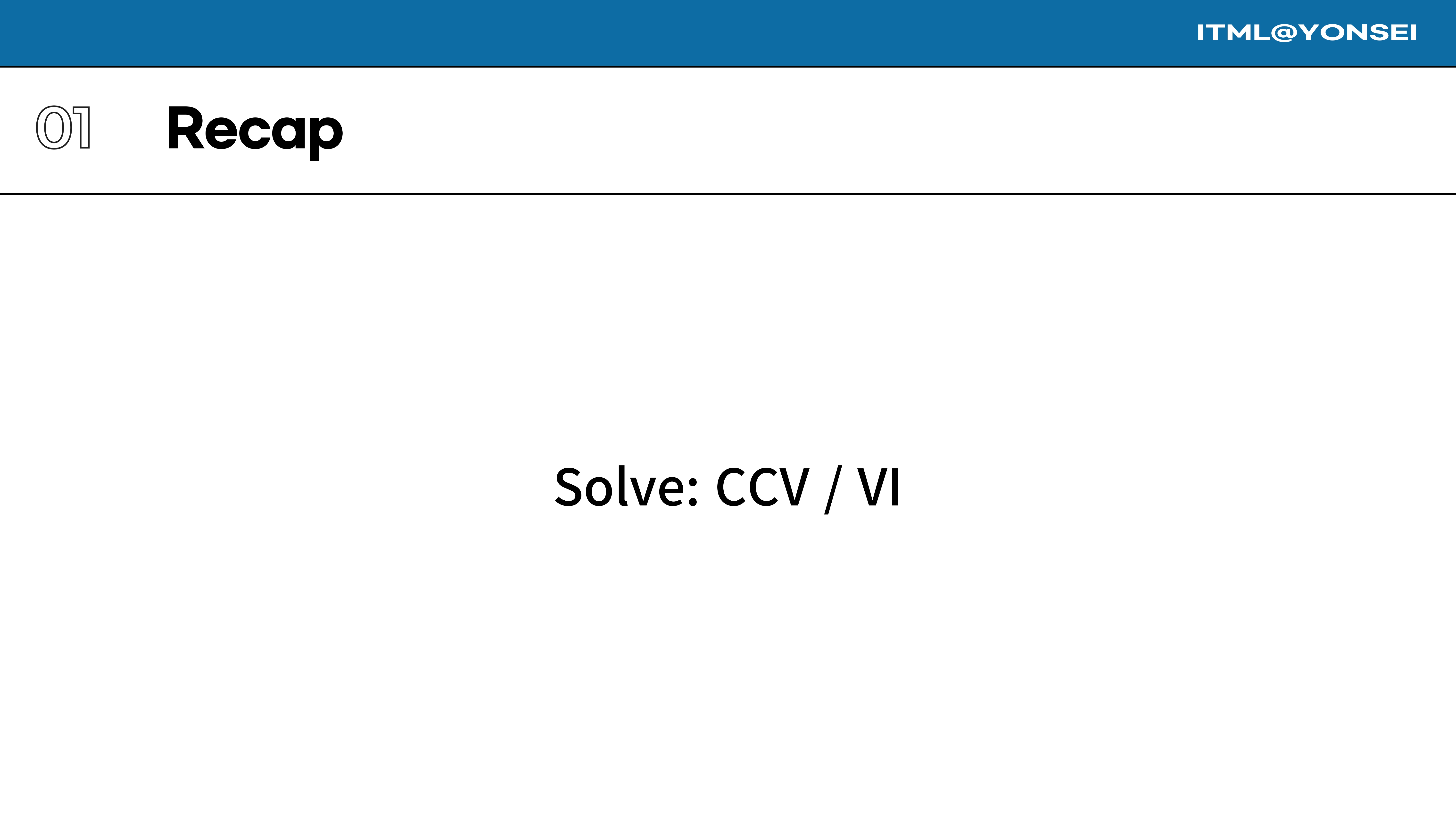
I’ll illustrate this with a simple task. Imagine you need to solve the division problem CCV / VI. For most people, this is not immediately obvious.

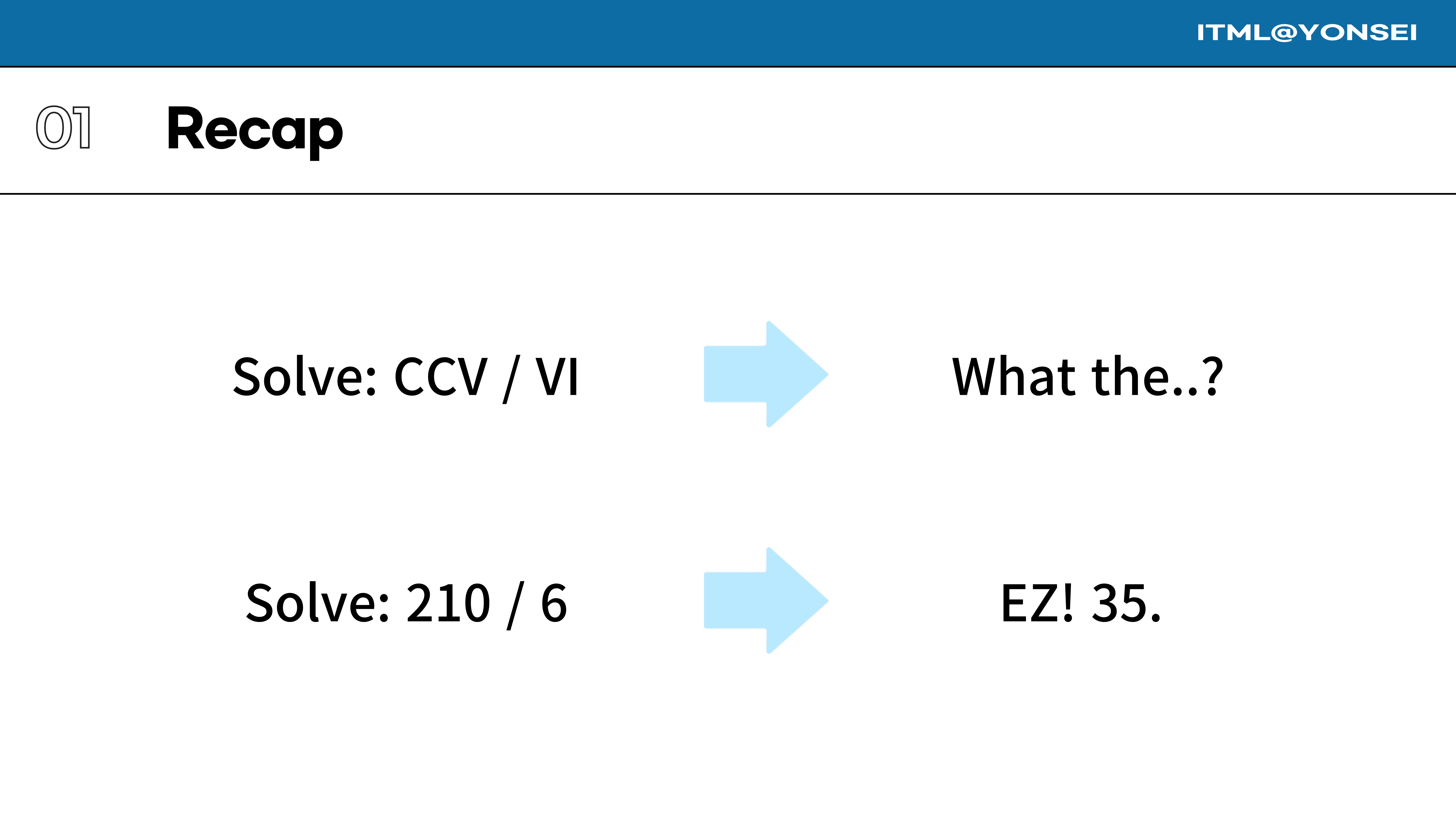
Now, consider this problem: 210 / 6. This is likely much easier, and you can quickly determine the answer is 35. The interesting part is that both problems represent the exact same calculation.

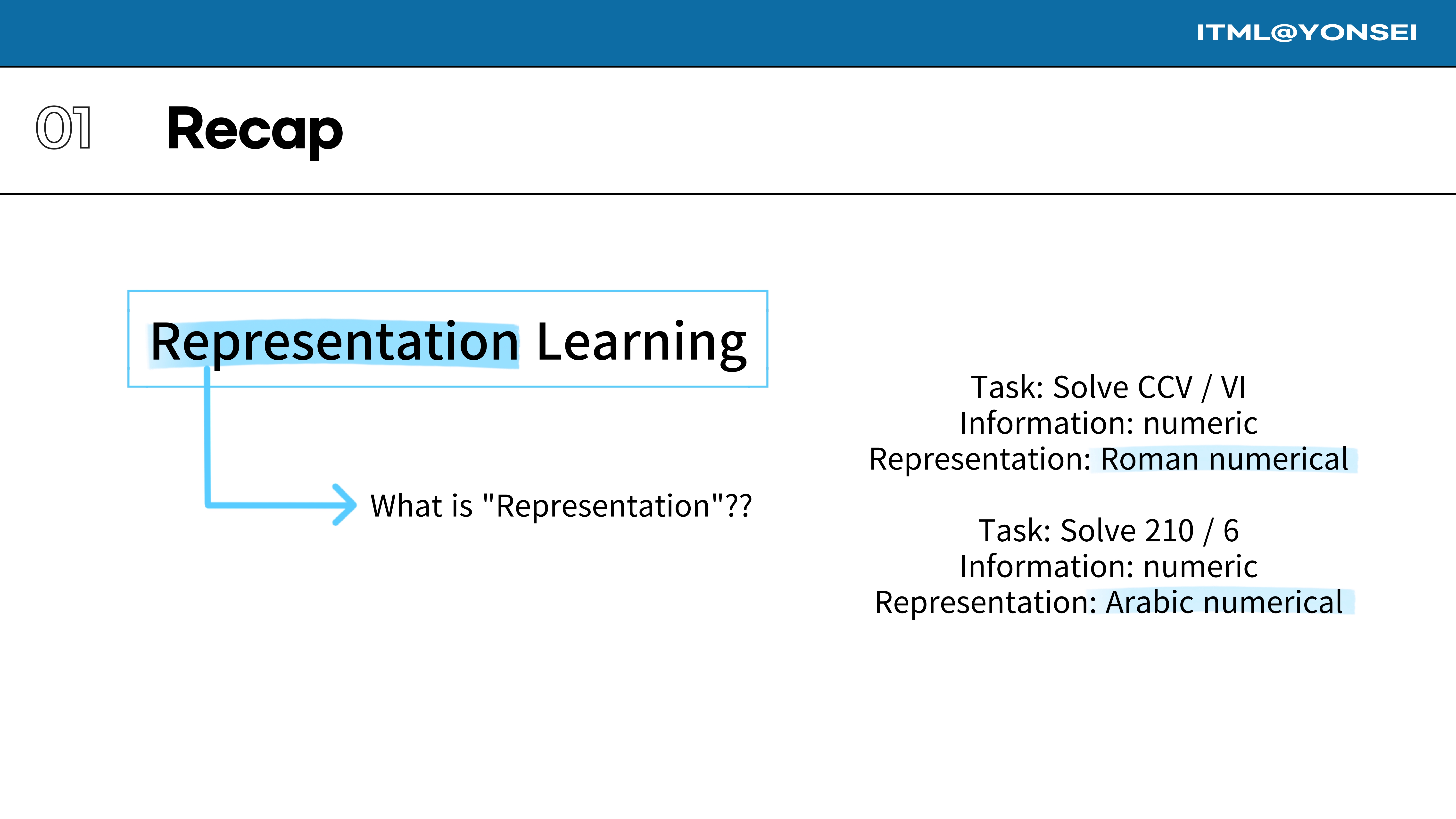
The key difference lies in the representation of the same numerical information. The first task used Roman numerals, while the second used Arabic numerals. The choice of representation dramatically changes the difficulty of the task.

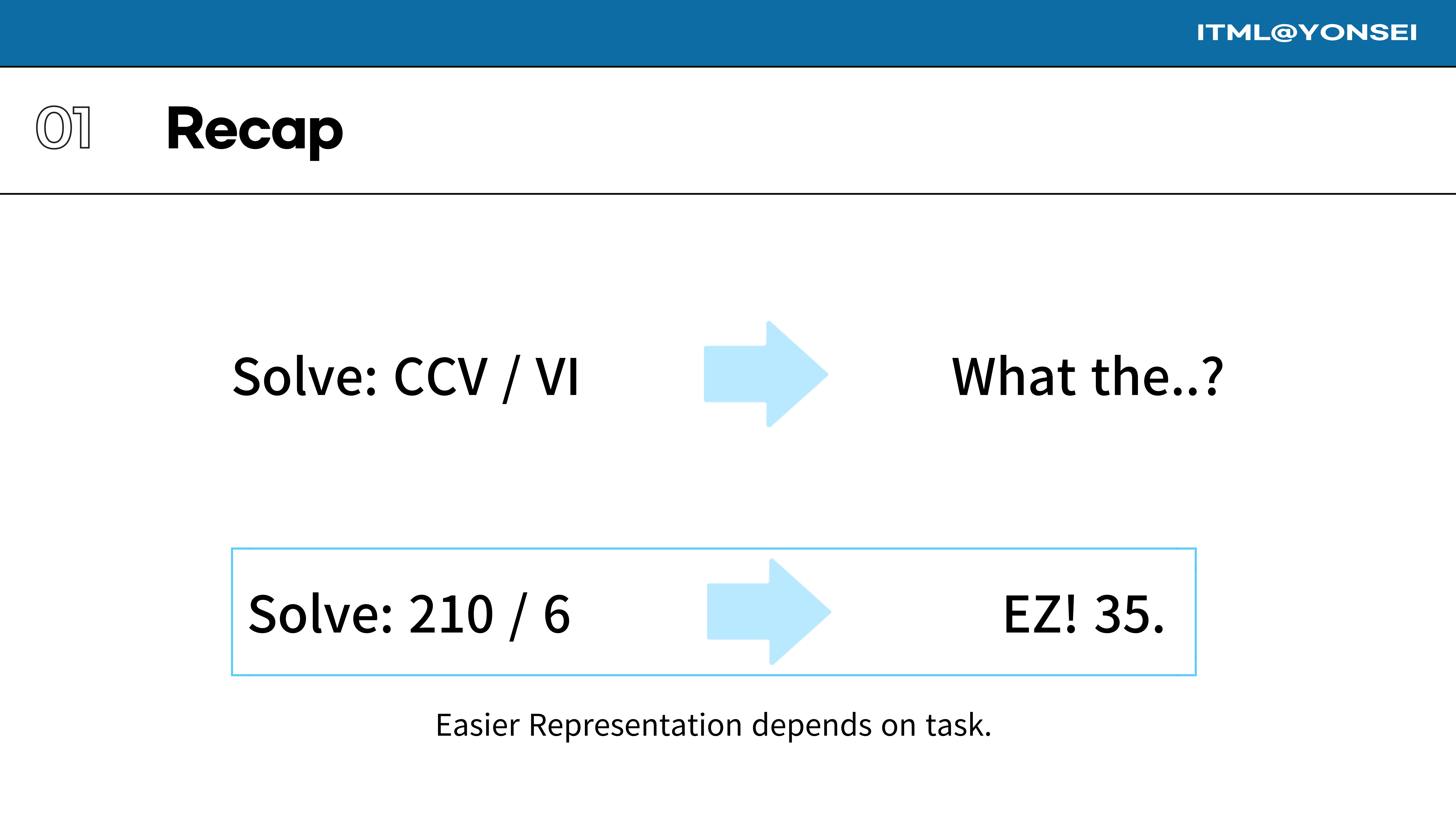
This analogy illustrates a critical point that is central to representation learning: the right representation can make a complex task much easier to solve.

To summarize this introductory point: the difficulty of many information processing tasks is highly dependent on how that information is represented.

So, the crucial question for us is: how can we obtain a “good representation” for various machine learning tasks? Today, I’ll focus on one prominent approach for achieving this: Self-Supervised Learning.

Self-Supervised Learning is a subset of the broader field of Representation Learning.

A primary motivation for the development of self-supervised methods is the immense cost and effort required to obtain large-scale labeled datasets for traditional supervised learning.

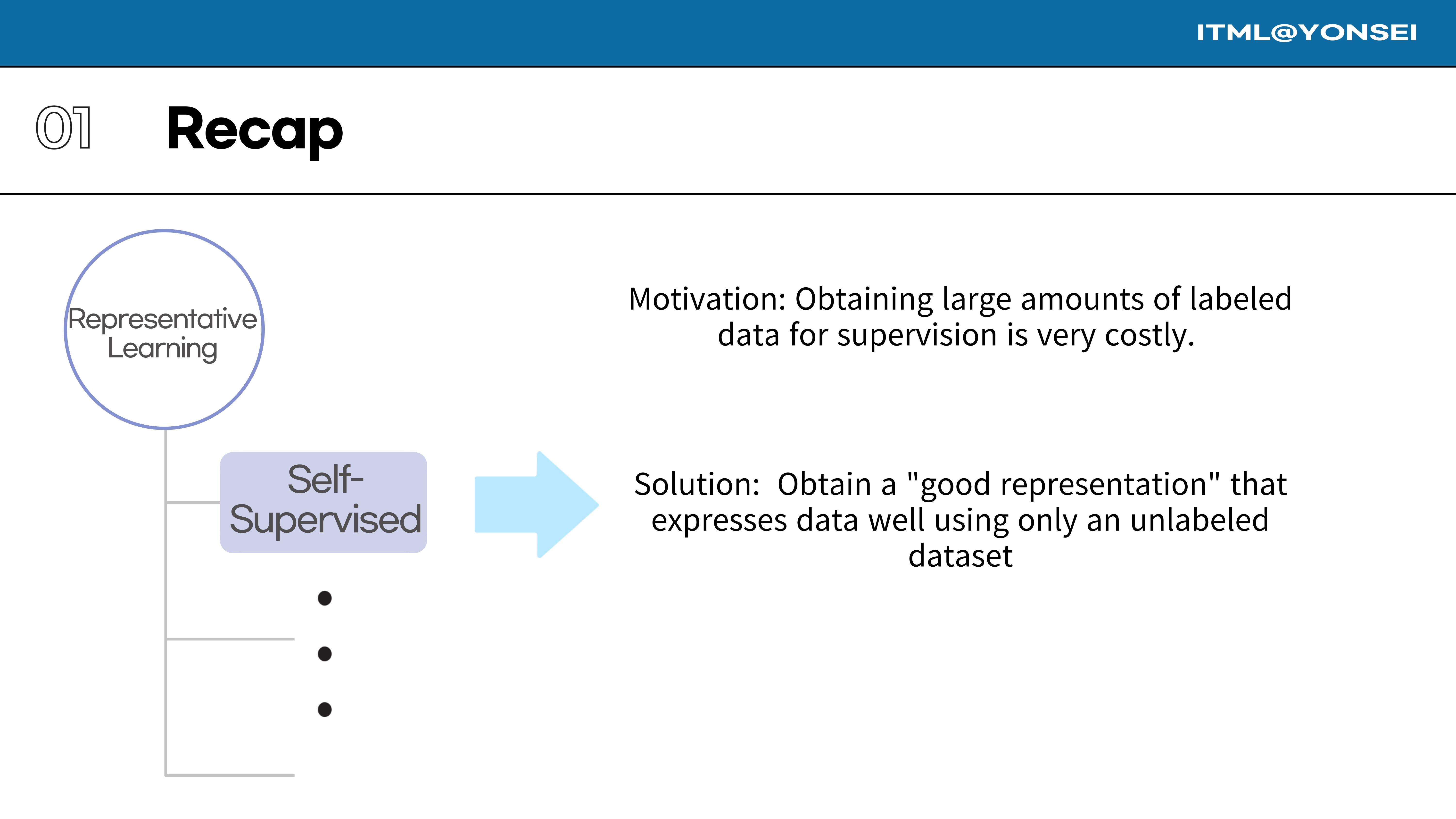
The solution that Self-Supervised Learning proposes is to find a way to learn a “good representation” that captures the essential features of the data using only an unlabeled dataset.

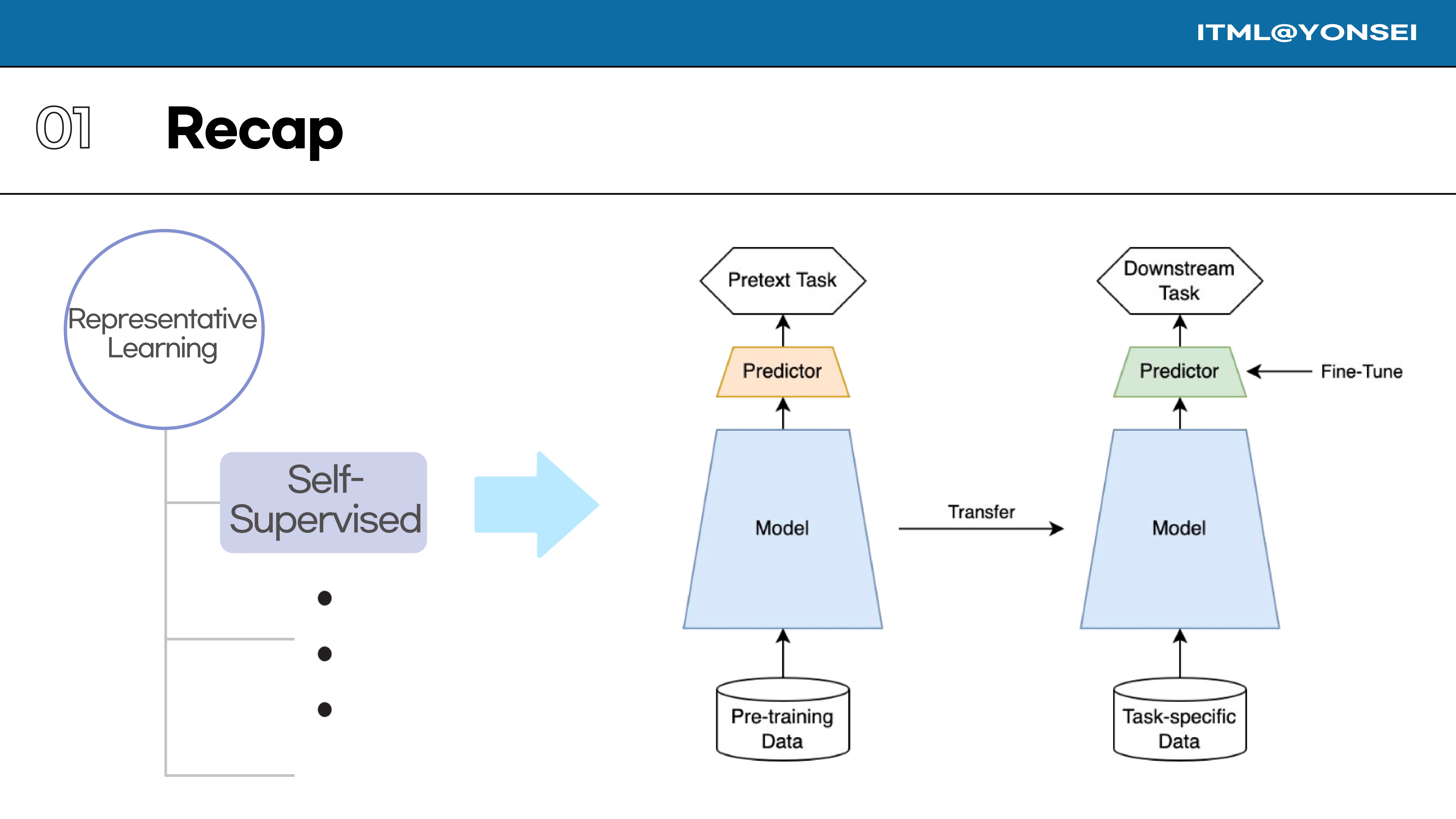
This slide illustrates the typical self-supervised learning pipeline. First, a model is trained on a “pretext task” using a large amount of unlabeled data. The learned model is then transferred and fine-tuned on a “downstream task” using task-specific (and often limited) labeled data.

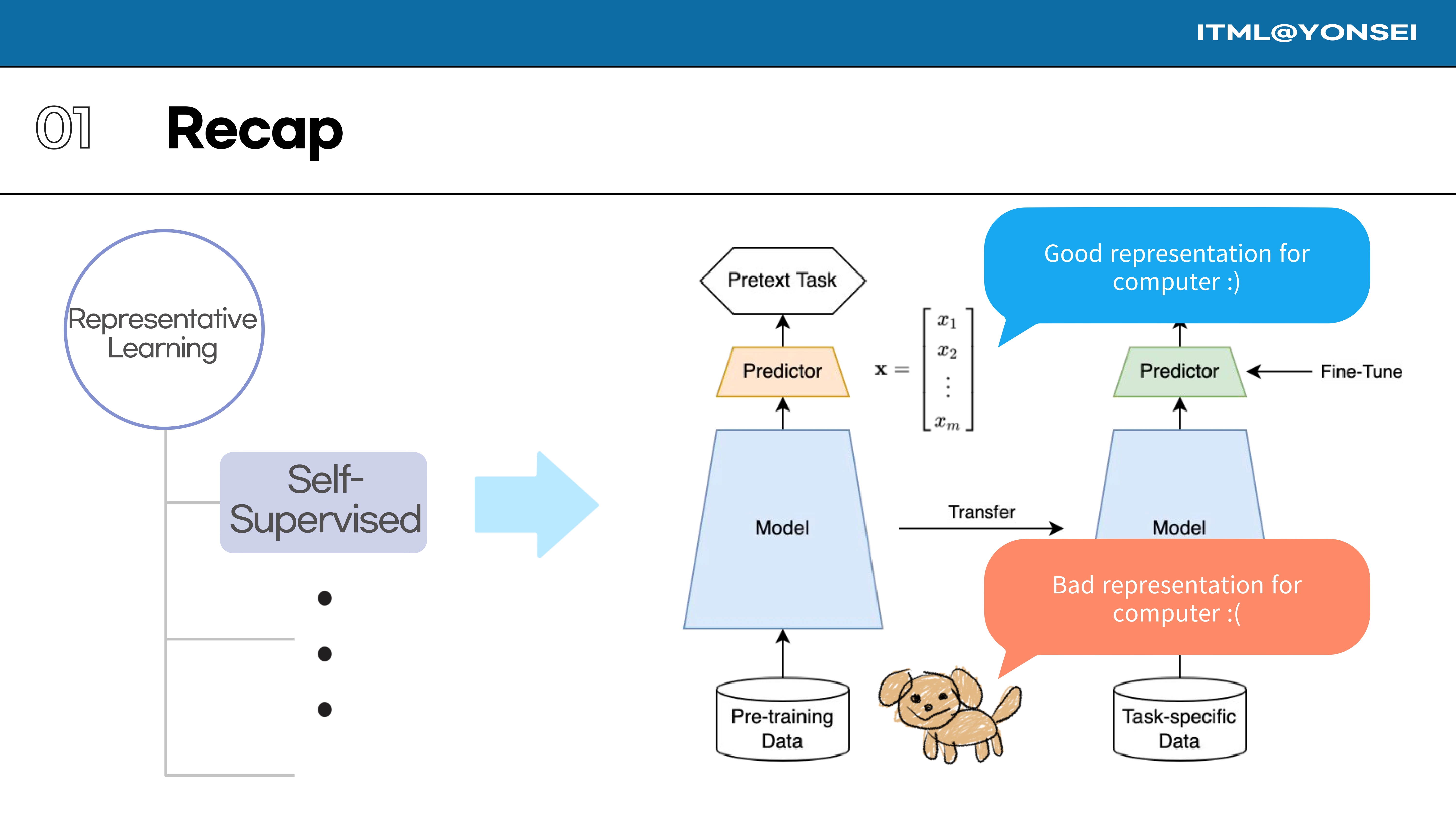
The goal of the pre-training stage is to transform raw data, which can be a poor representation for a computer (like a raw image of a dog), into a feature vector that is a much better representation for downstream tasks.

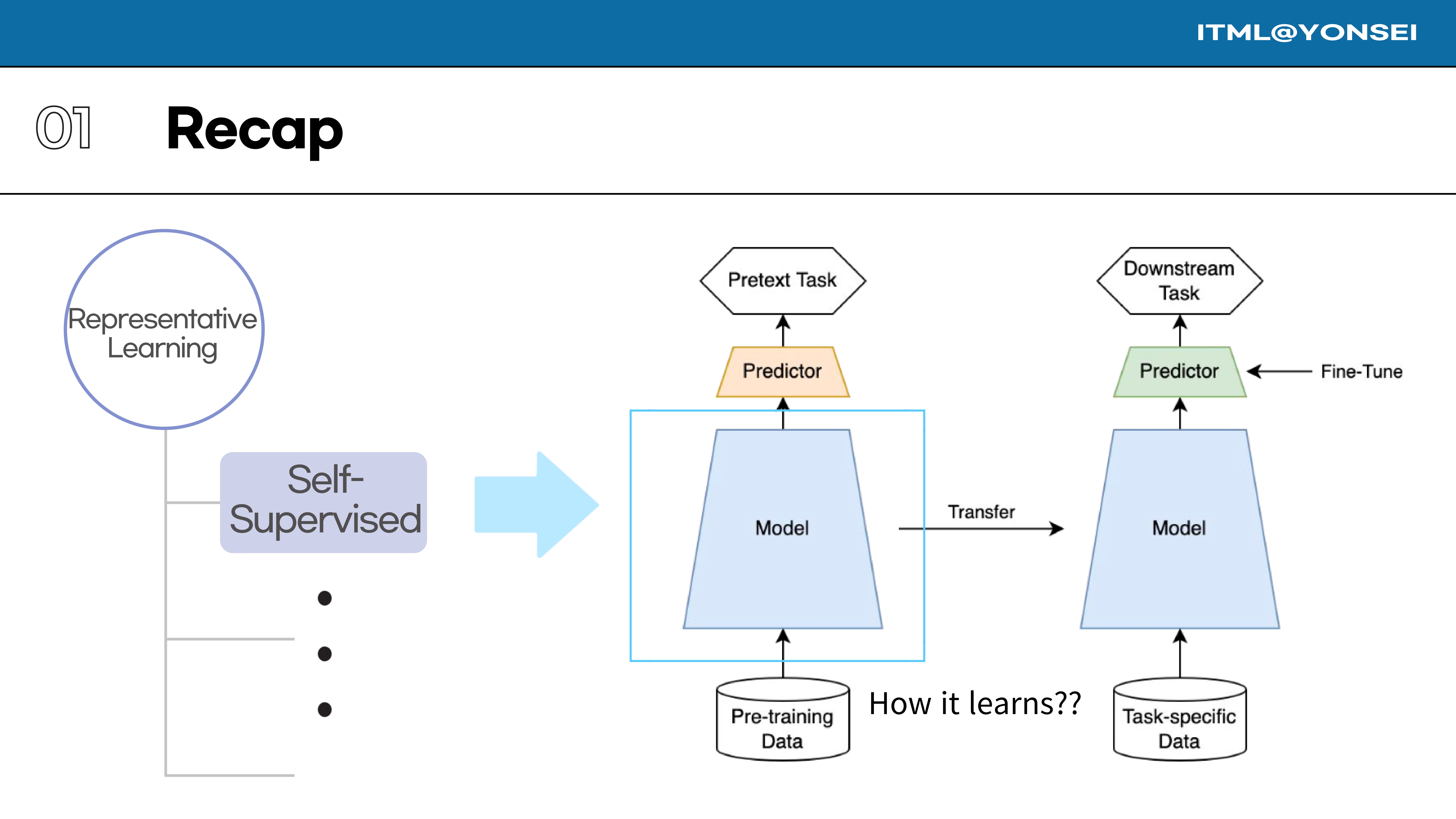
The central question this paper investigates is the pre-training step: how exactly does the model learn a good representation from unlabeled data?

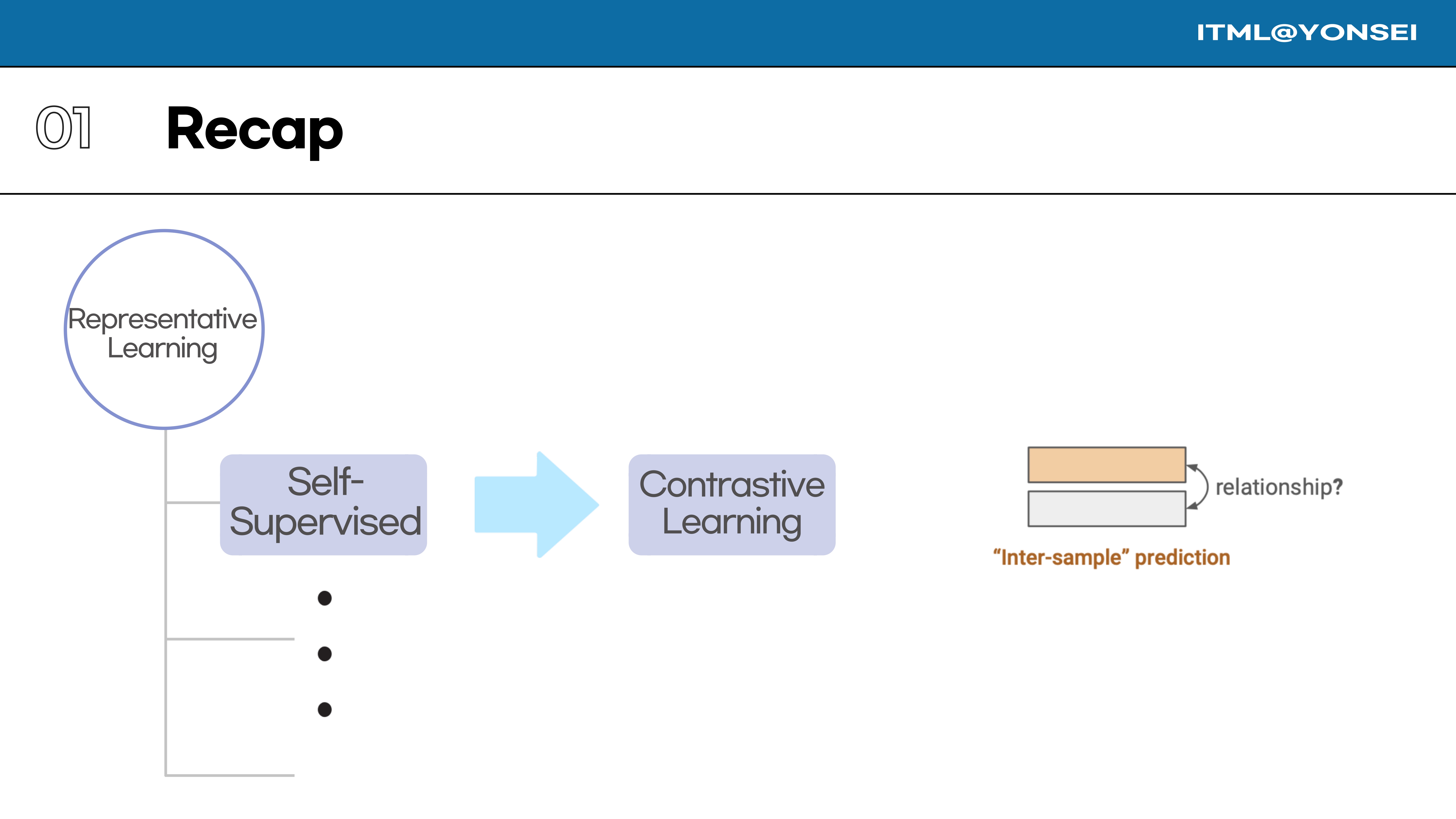
Within the realm of Self-Supervised Learning, I will now narrow the focus to Contrastive Learning. This approach is based on making “inter-sample” predictions.

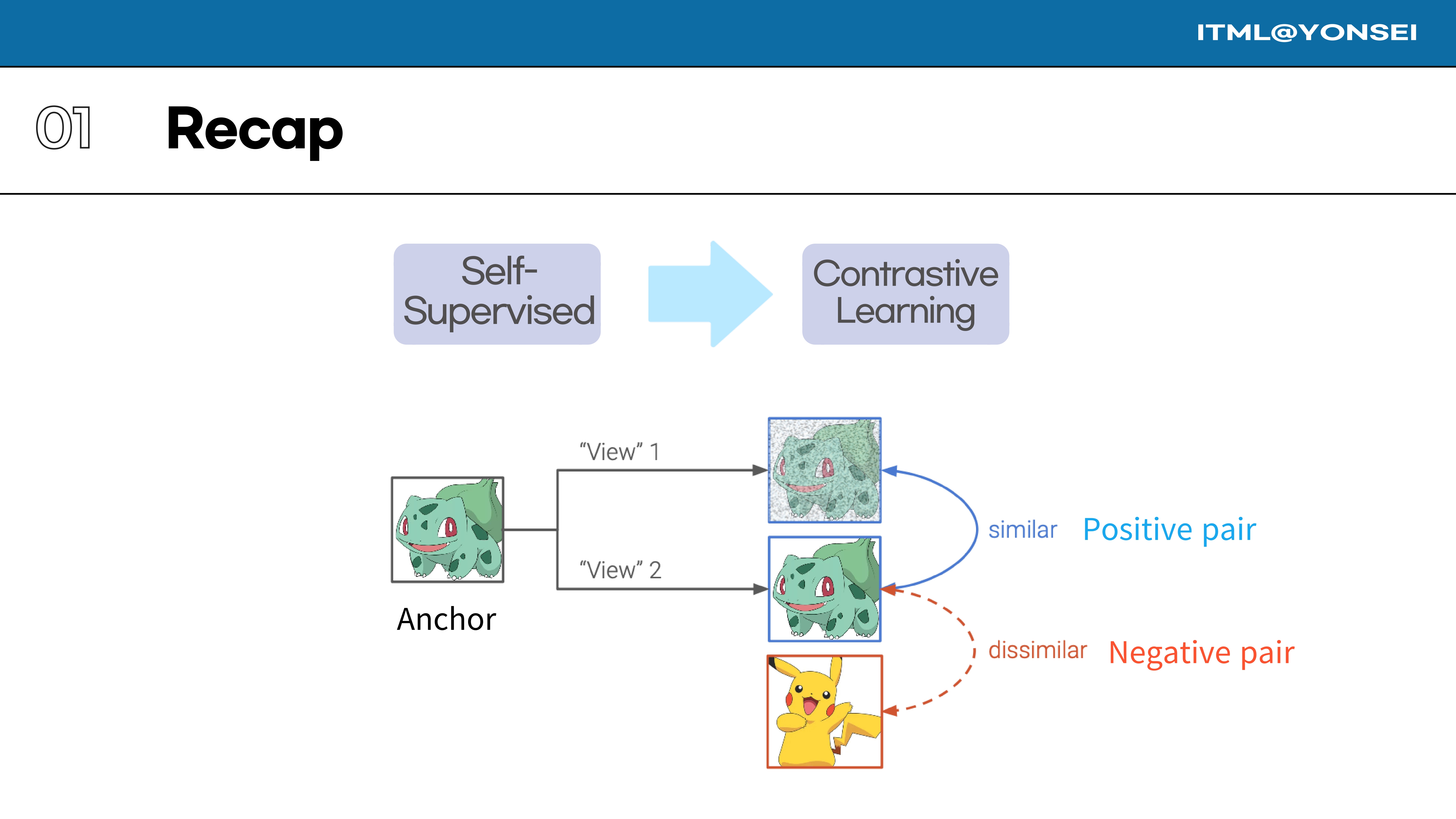
Here is the core mechanic of contrastive learning. We start with an “anchor” image. We create two different augmented versions, or “views,” of this anchor, which form a “positive pair.” We then contrast this with a “negative pair,” which is formed by the anchor and a view from a completely different image.

In summary, the objective of contrastive learning is to learn effective representations by mapping similar data points close to each other in the representation space, while simultaneously pushing dissimilar data points far apart.

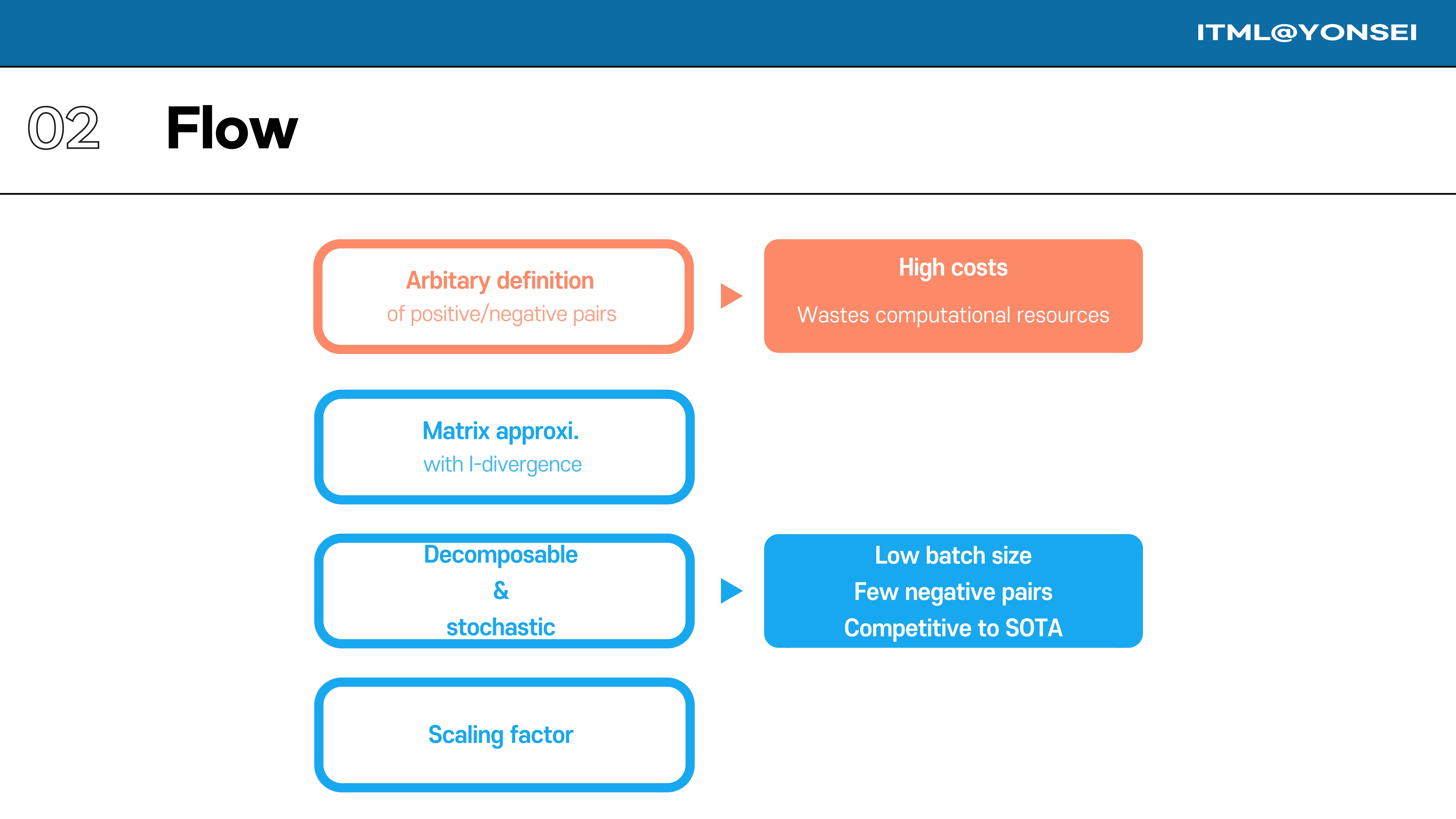
This slide outlines the flow of the main arguments in this review. I’ll begin by discussing the high computational costs that arise from the conventional definition of positive and negative pairs. Then, I will introduce the paper’s proposed method, which uses matrix approximation with I-divergence to create a decomposable and stochastic loss, ultimately achieving competitive results with a low batch size and fewer negative pairs.

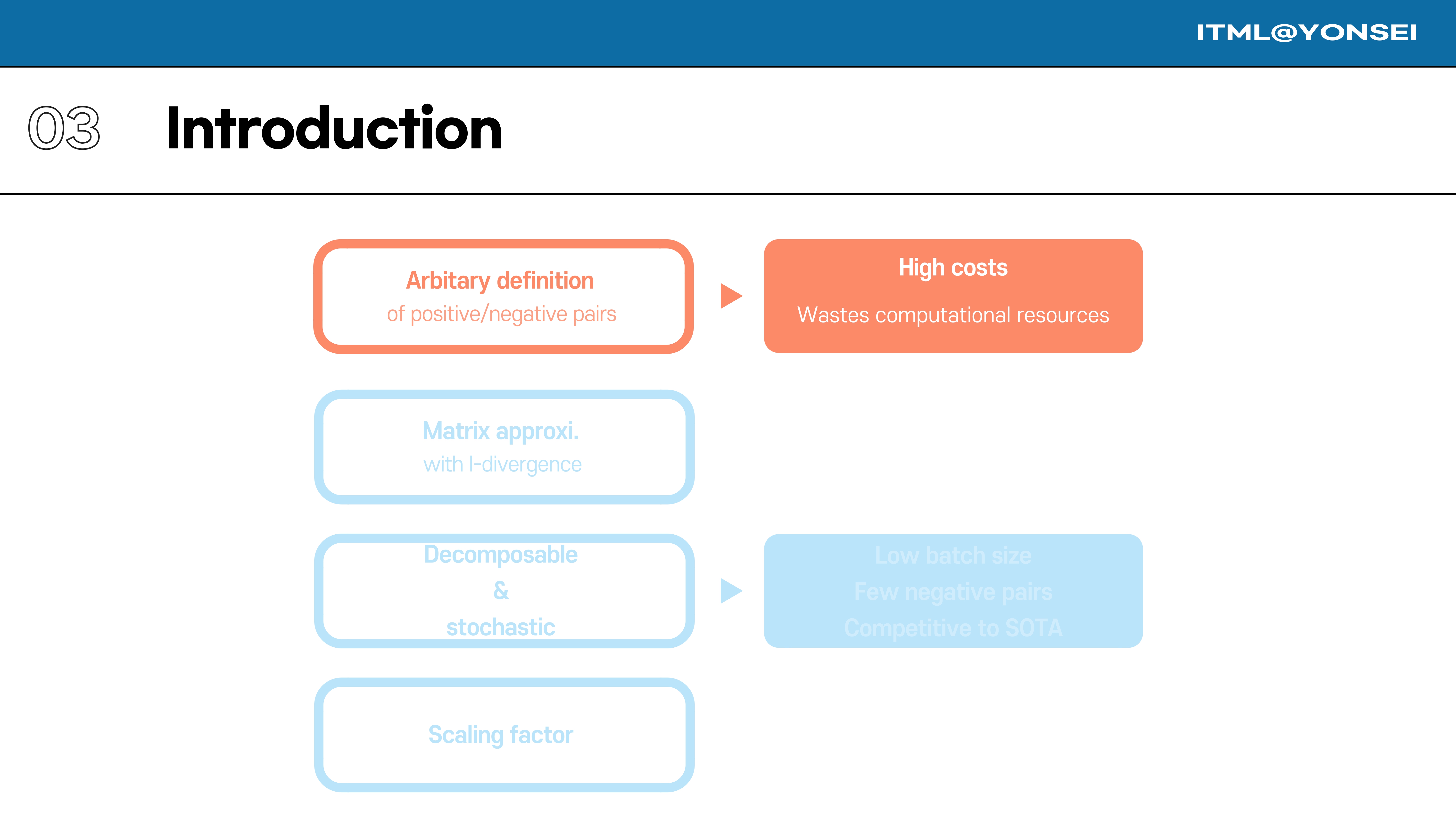
Now, we move from the recap to the main introduction of the paper’s contribution.

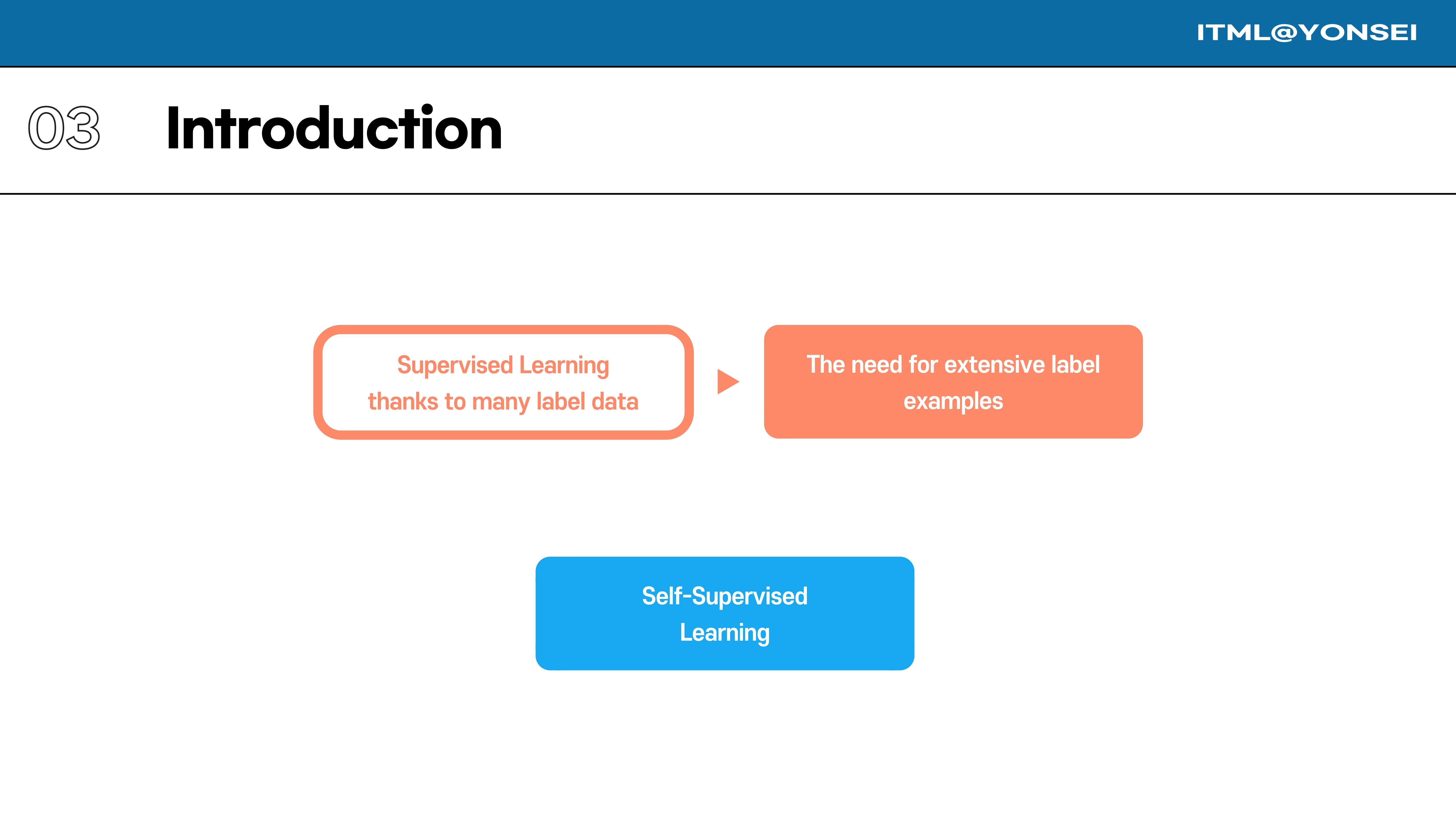
The core problem is that while supervised learning is effective, it depends on having extensive labeled data. Self-Supervised Learning is the alternative we are exploring.

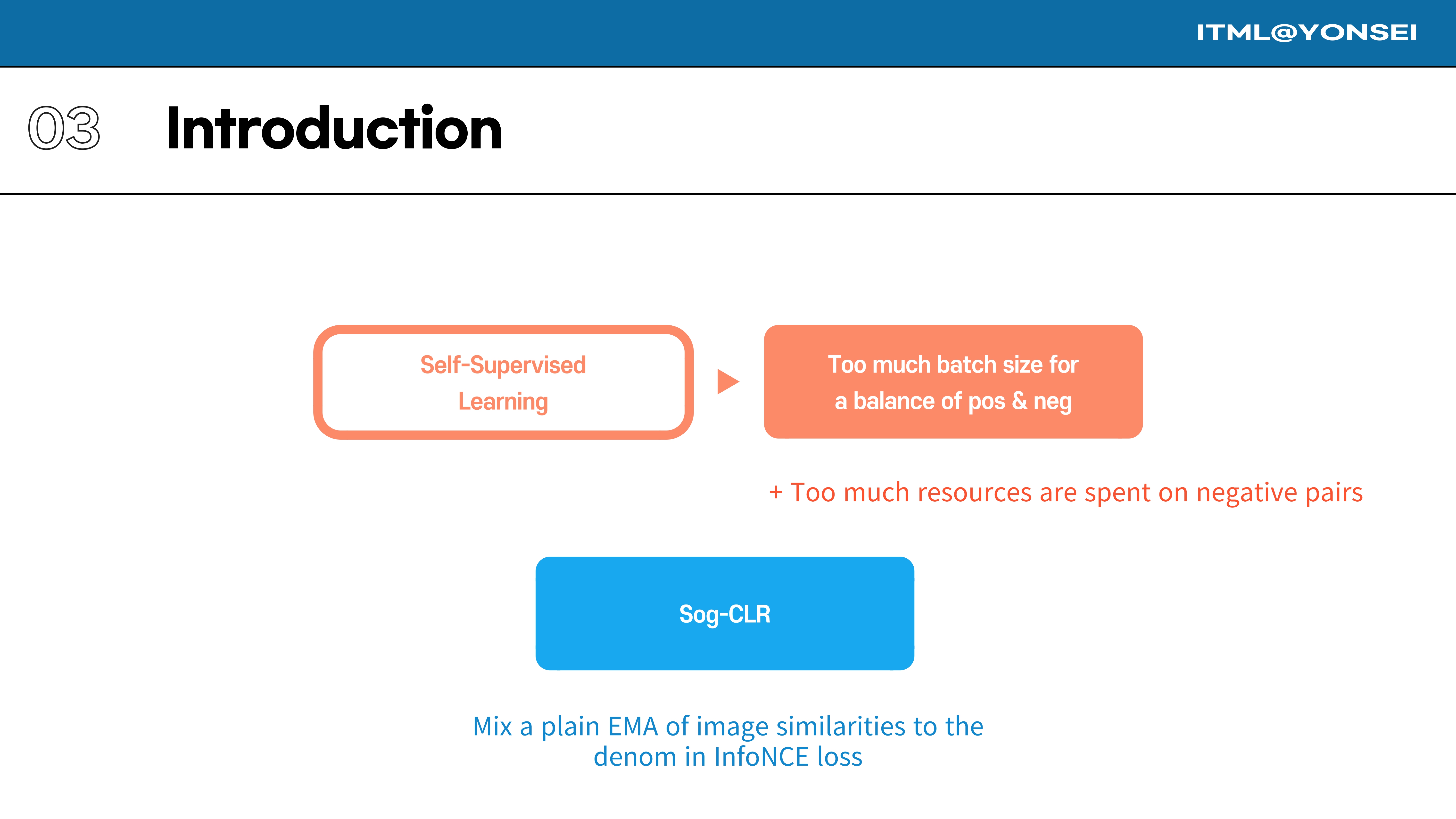
However, popular contrastive learning methods like SimCLR require very large batch sizes to ensure a sufficient balance of positive and negative examples. This expends a large amount of computational resources, particularly on the negative pairs. A method called Sog-CLR attempted to address this by mixing an EMA of image similarities into the denominator of the InfoNCE loss.

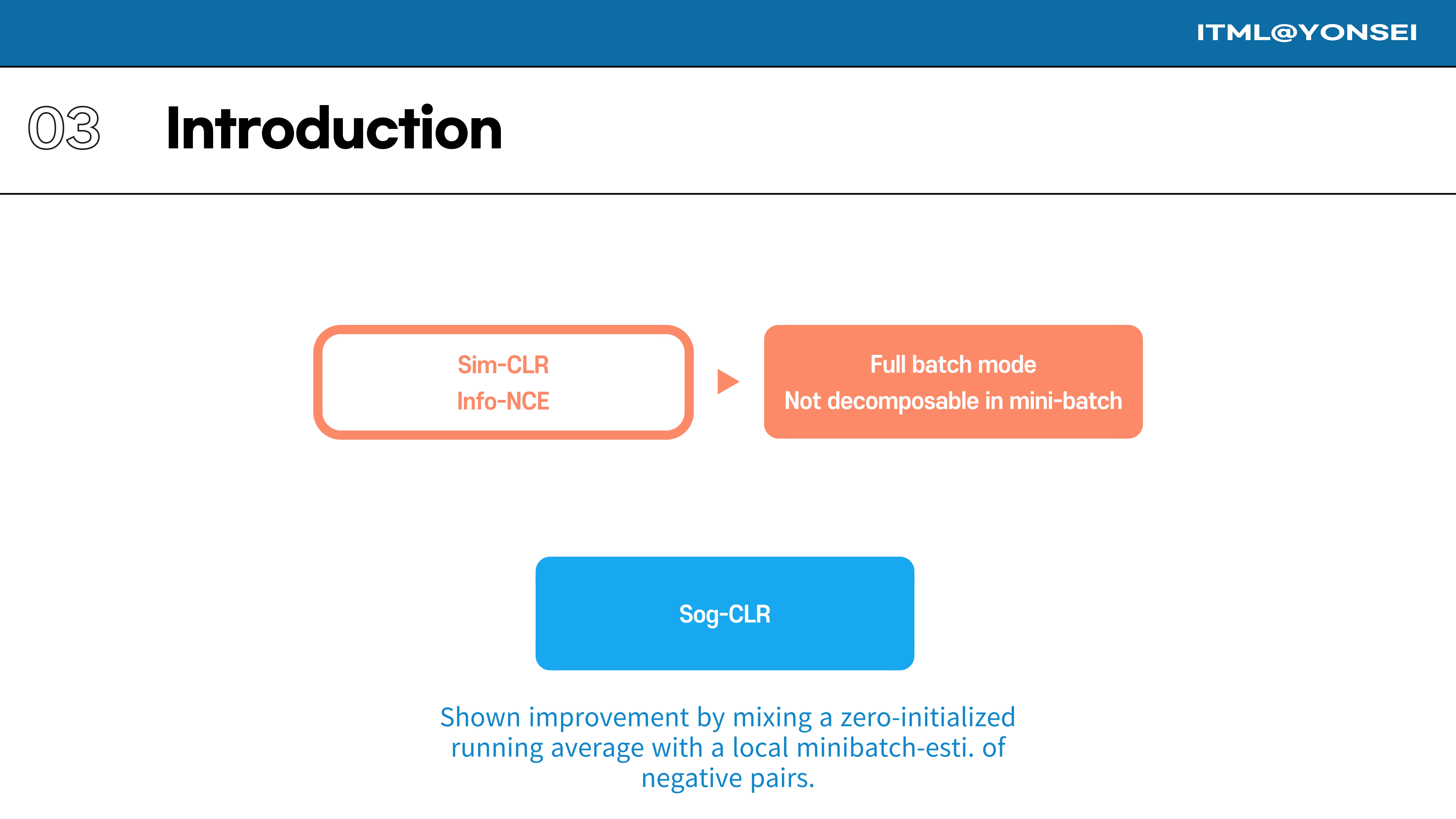
To be more specific, SimCLR’s InfoNCE loss operates in a full-batch mode, which is not decomposable in a mini-batch setting. Sog-CLR showed improvement by incorporating a running average for the negative pair estimations.

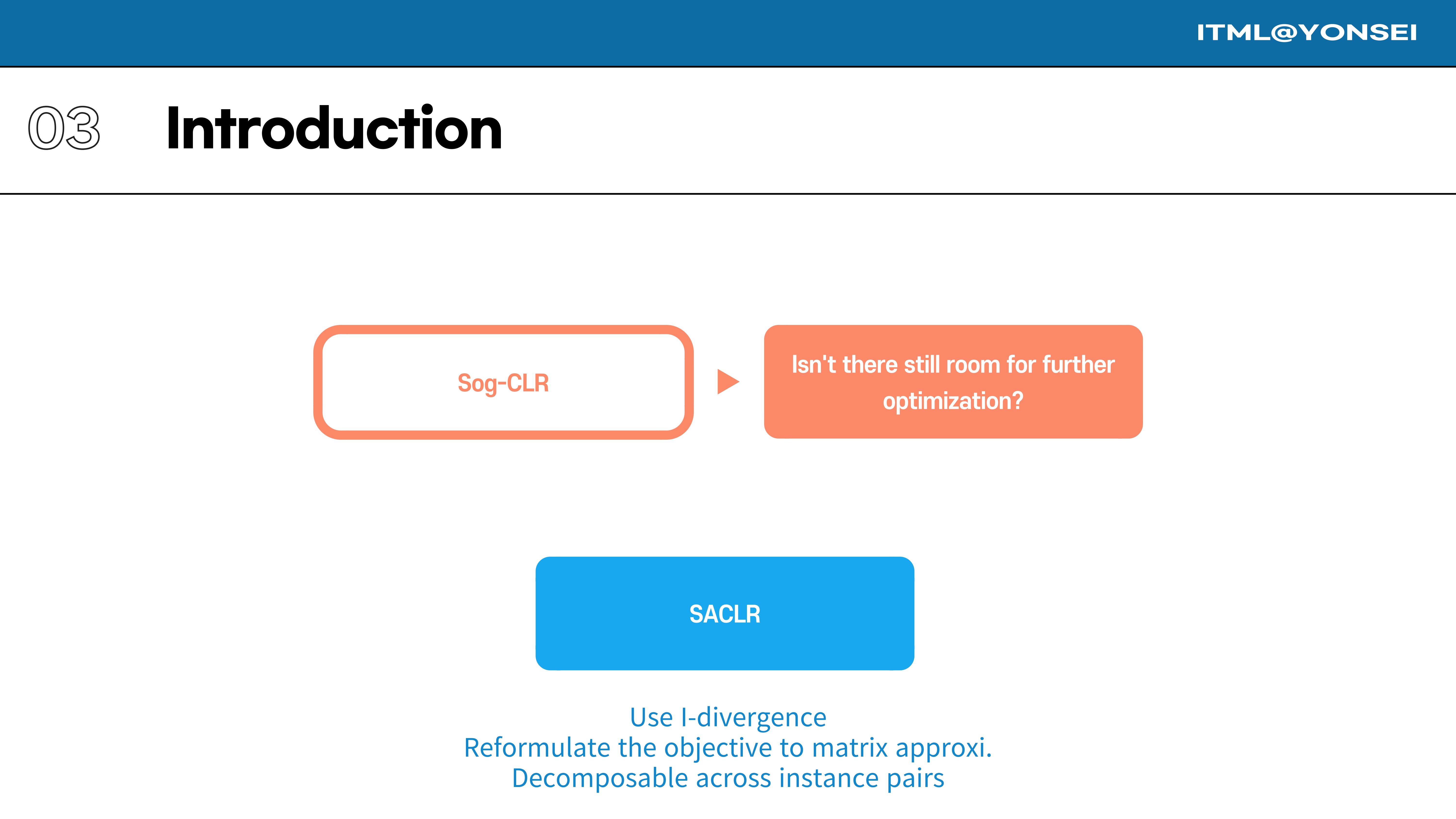
This paper poses the question: even with Sog-CLR’s improvements, is there still room for further optimization? It introduces SACLR, a method that uses I-divergence to reformulate the objective into a matrix approximation problem that is decomposable across instance pairs.

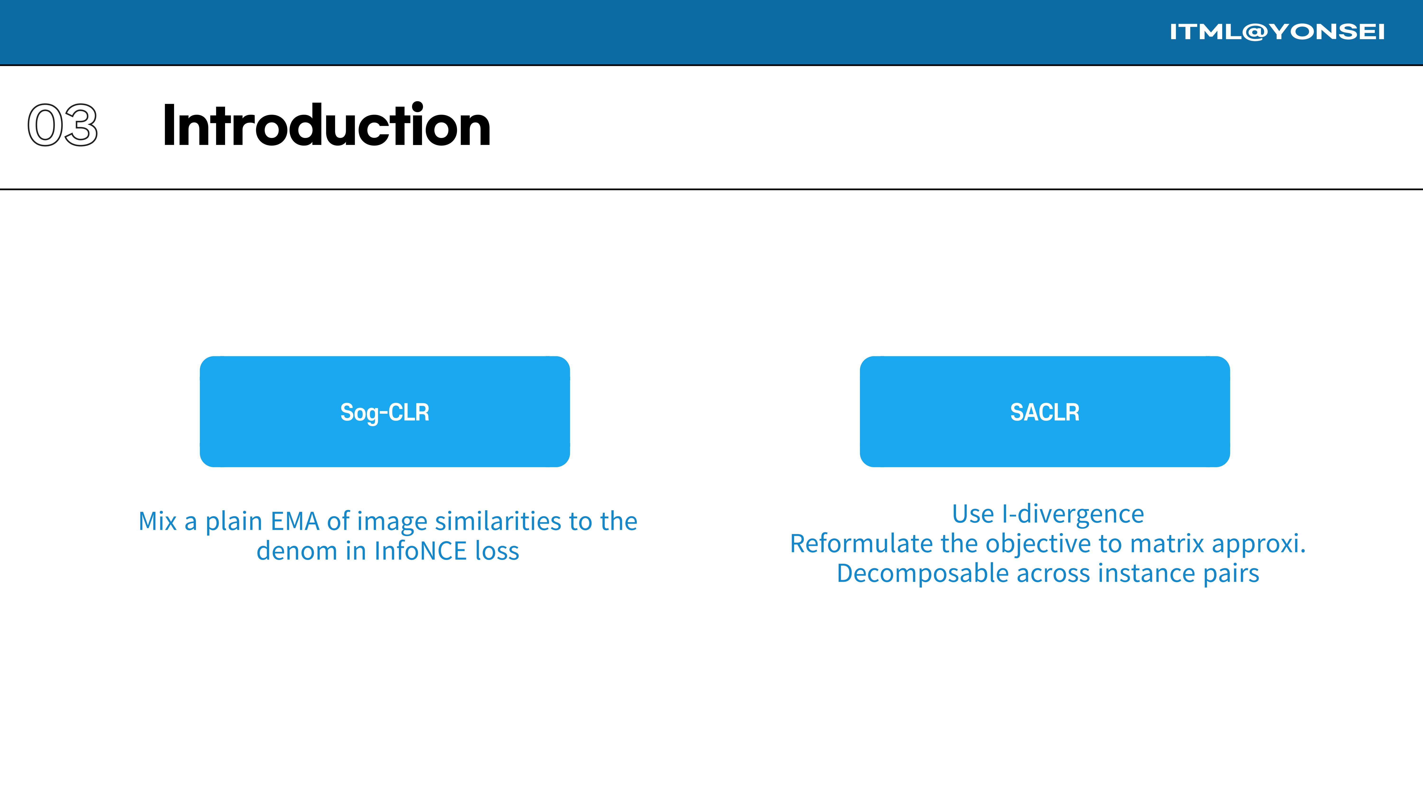
The key idea behind SACLR is this reformulation using I-divergence, which allows the objective to be decomposed and approximated stochastically. This is presented as an advancement over Sog-CLR’s EMA mixing approach.

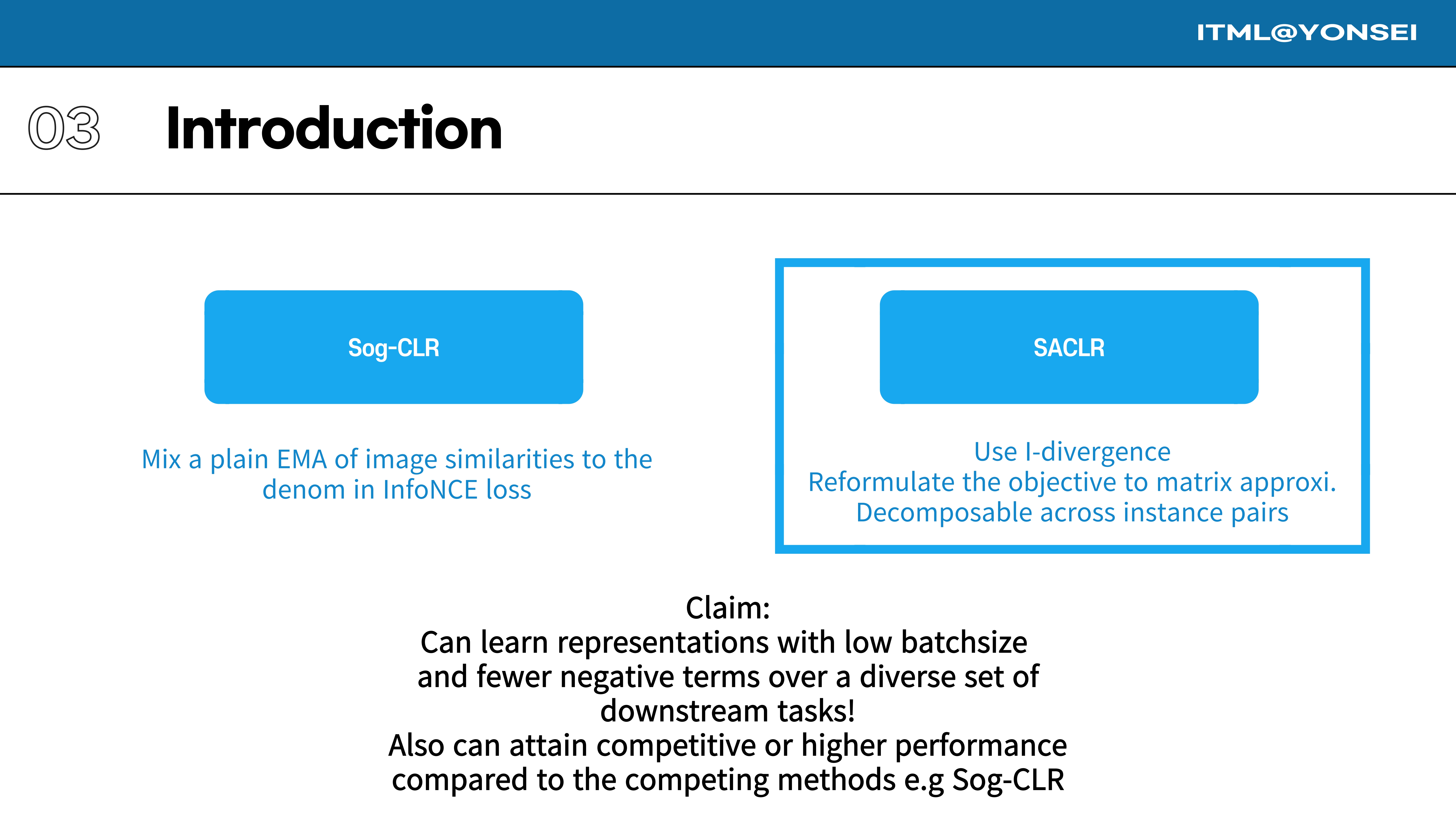
The paper’s central claim is that its method, SACLR, can learn high-quality representations with a small batch size and very few negative pairs. While reviewers found the core idea of tackling the large batch size problem to be an interesting and valuable contribution, and saw the novel formulation inspired by Stochastic Cluster Embedding as a strength, they heavily scrutinized the experimental evidence supporting these claims.

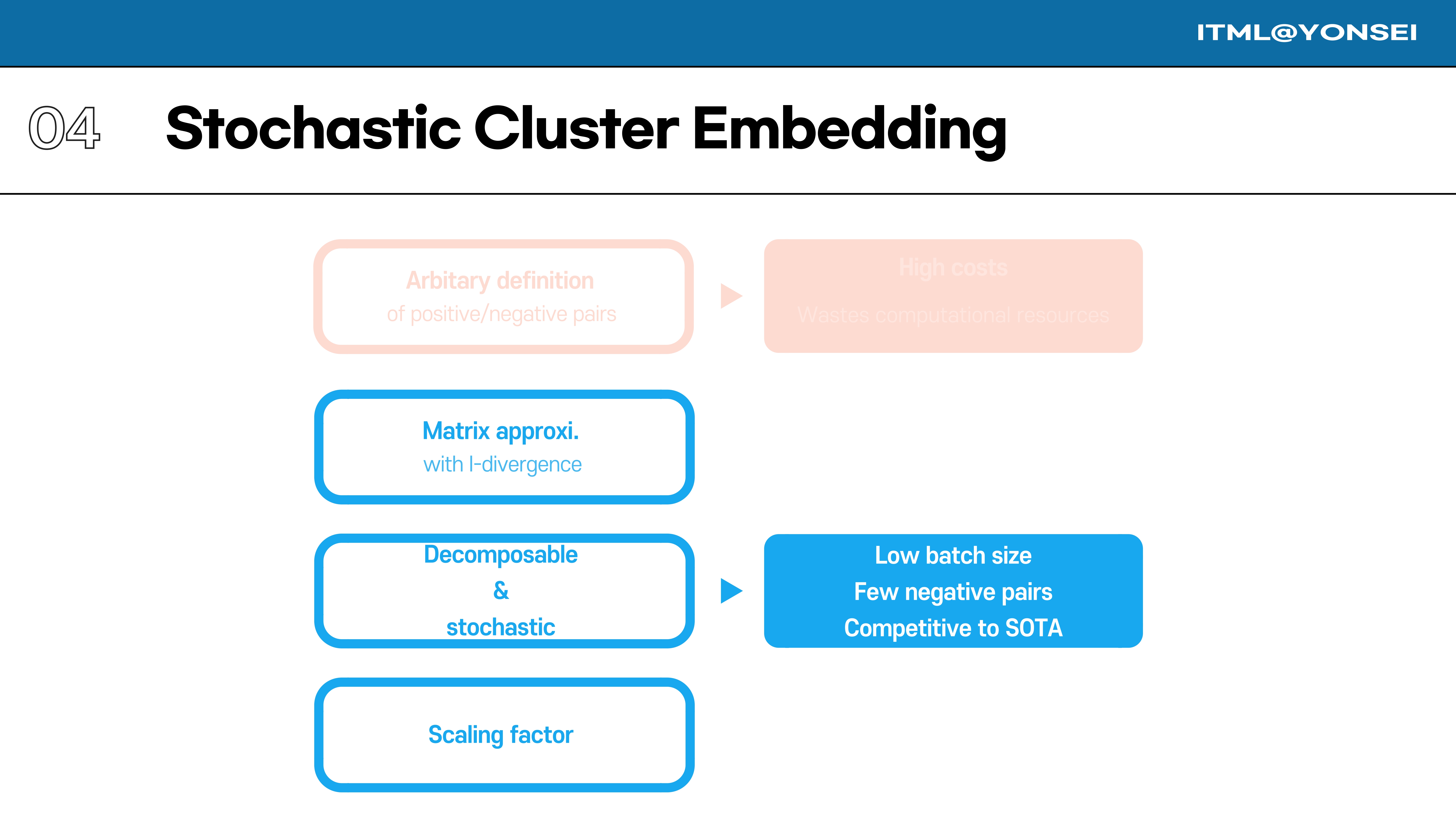
To understand SACLR, we first need to look at its theoretical foundation: Stochastic Cluster Embedding (SCE). I will now detail the matrix approximation with I-divergence that underpins the method.

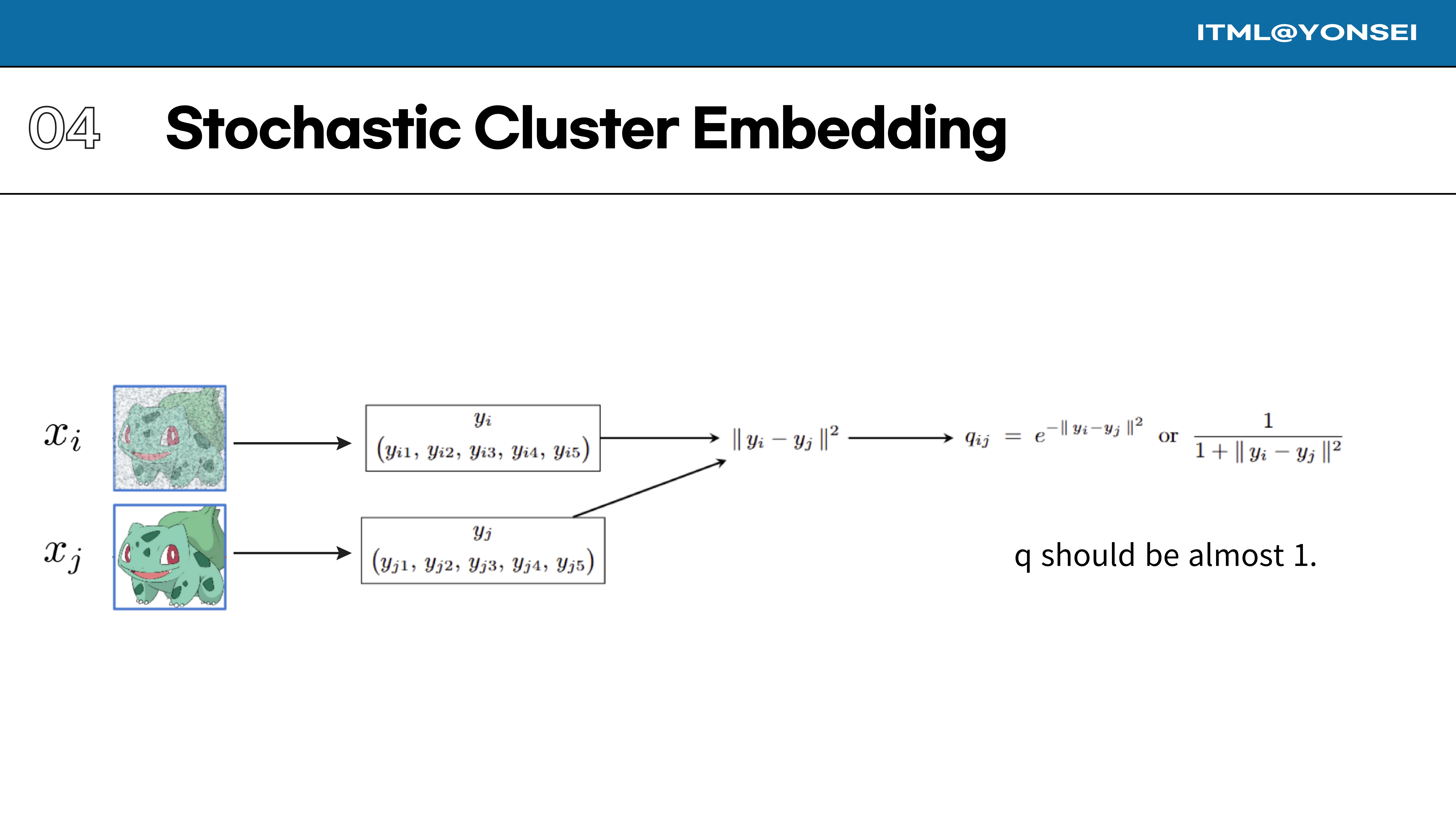
In SCE, we have embedded data points, like $y_i$ and $y_j$. We define a similarity kernel $q_{ij}$ between these points in the embedded space, typically using a Gaussian or a Student’s t-distribution kernel. This value should be close to 1 for similar points.

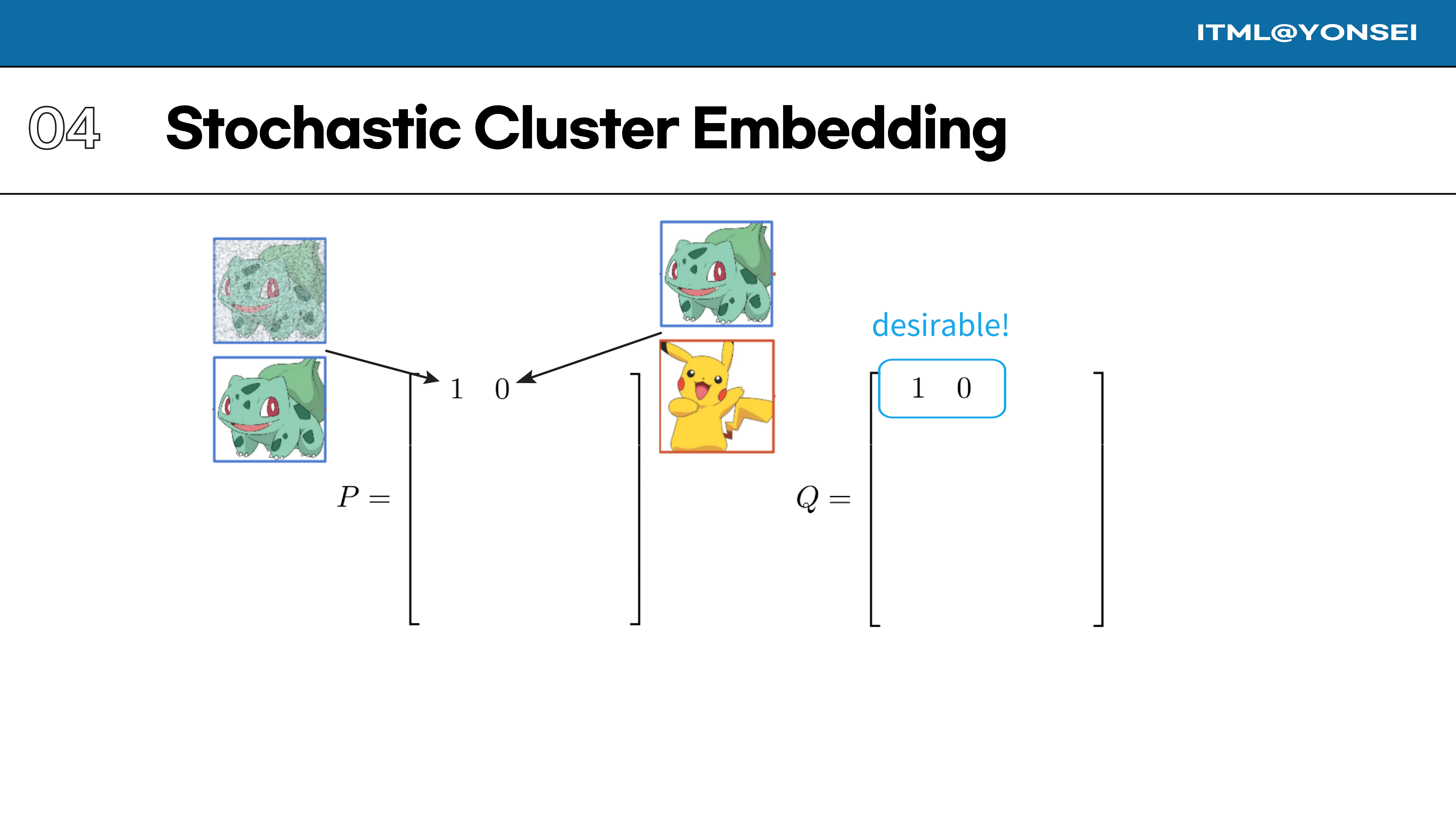
We also define a target similarity matrix, P, which represents the desired similarities in the embedded space. For example, perfectly clustered data would have a block-diagonal P matrix.

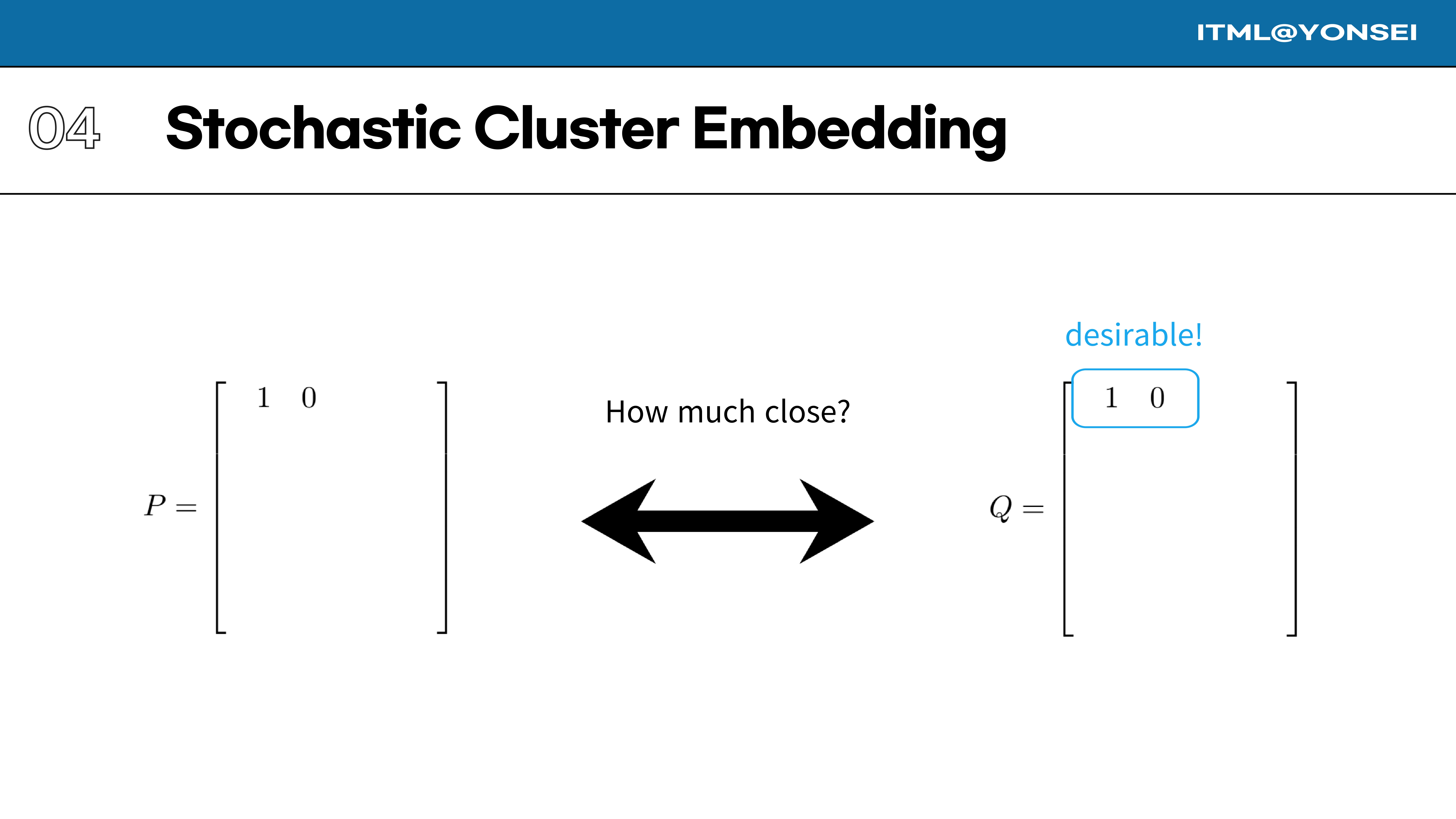
The goal is to make the learned similarity matrix Q as close as possible to our desirable target matrix P. The question is, how do we measure this closeness?

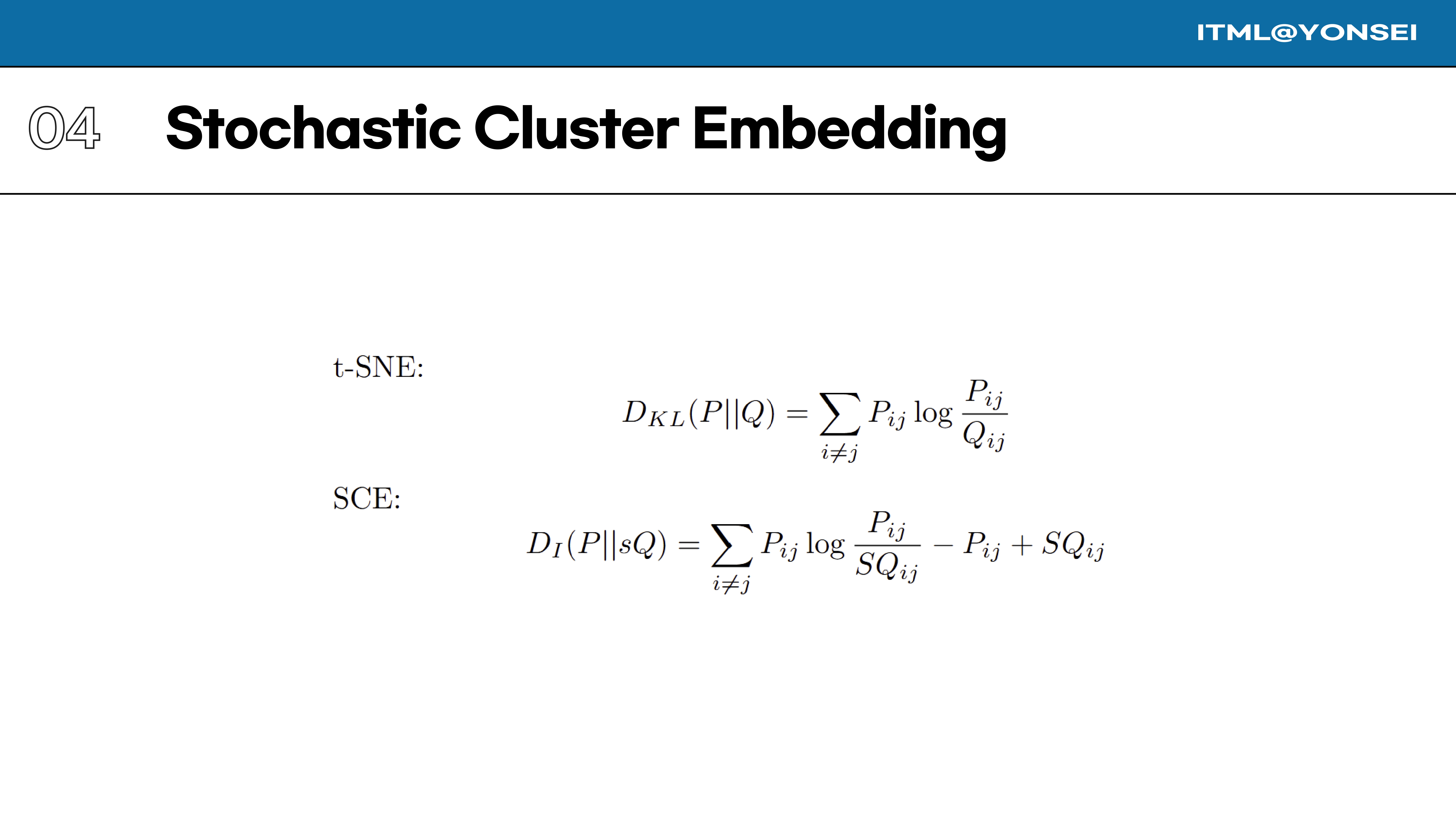
This is where the choice of divergence metric is crucial. t-SNE uses the KL-divergence. In contrast, SCE uses the I-divergence, which includes an additional scaling factor ’s’ and linear terms.

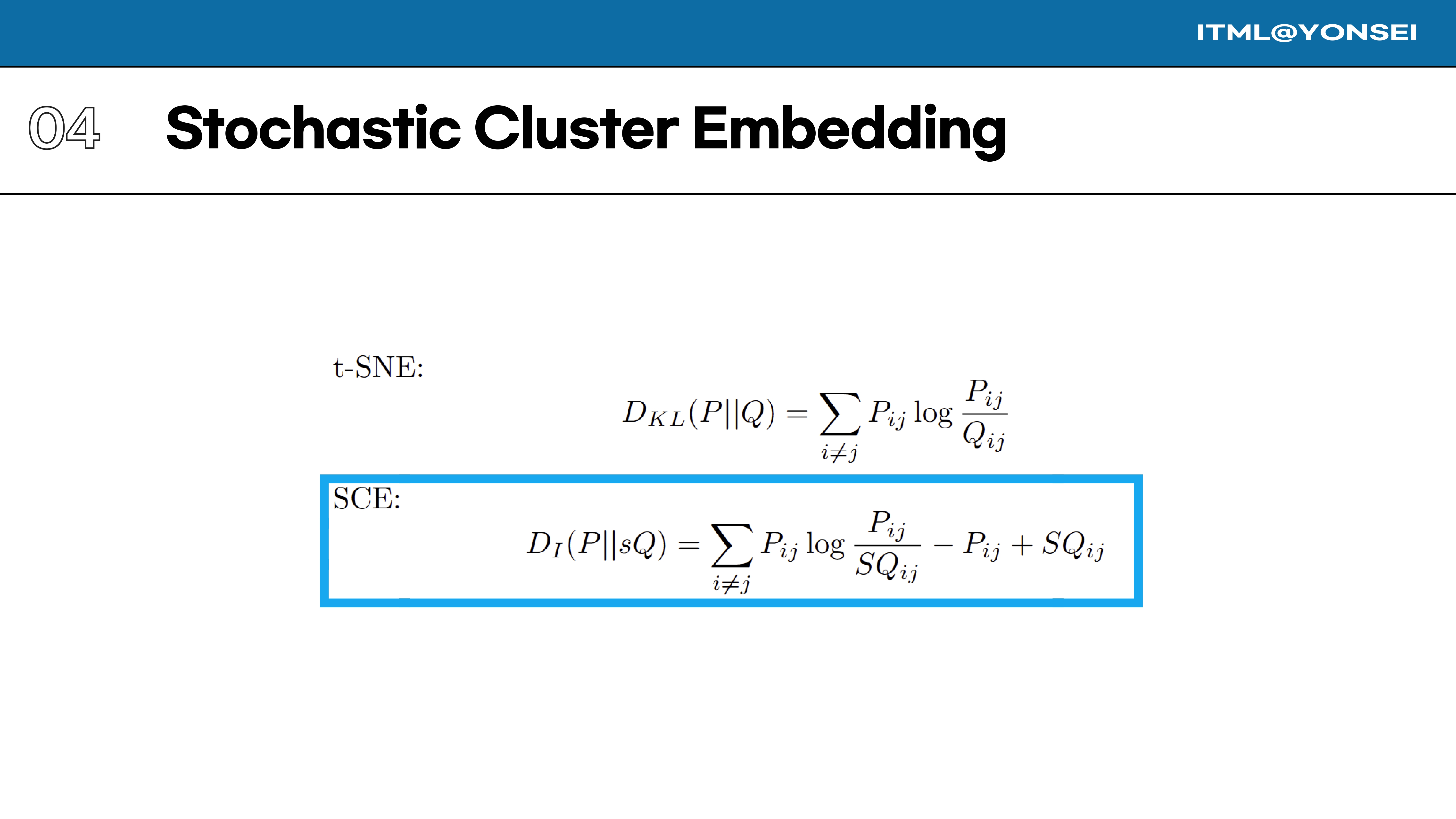
This slide highlights the formulas for both KL-divergence, used in t-SNE, and the I-divergence with a scaling factor, used in SCE.

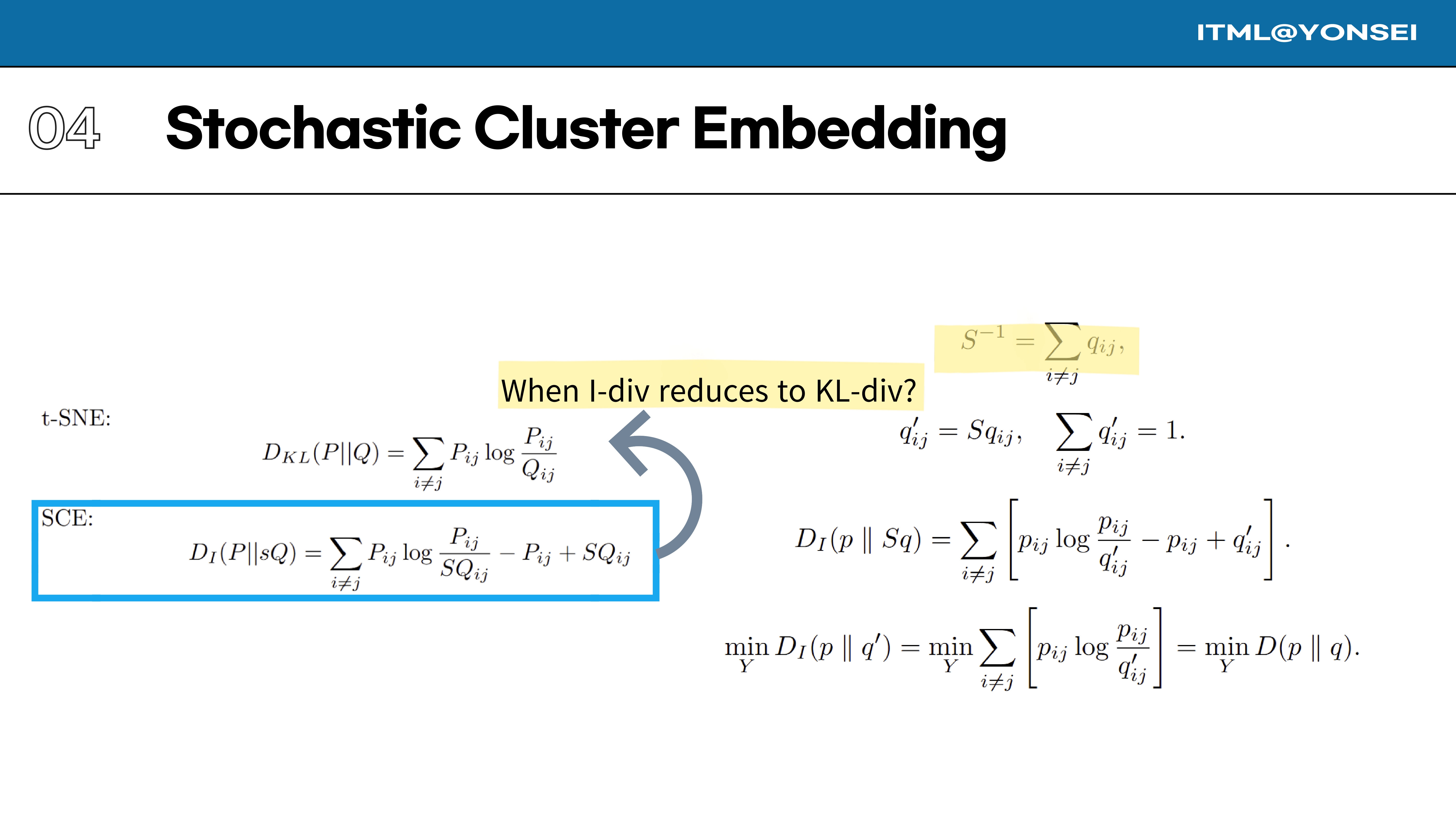
An important property is that the I-divergence can reduce to the KL-divergence. This happens if the scaling factor ’s’ is set to be the inverse of the sum of all kernel similarities, effectively normalizing the Q matrix.

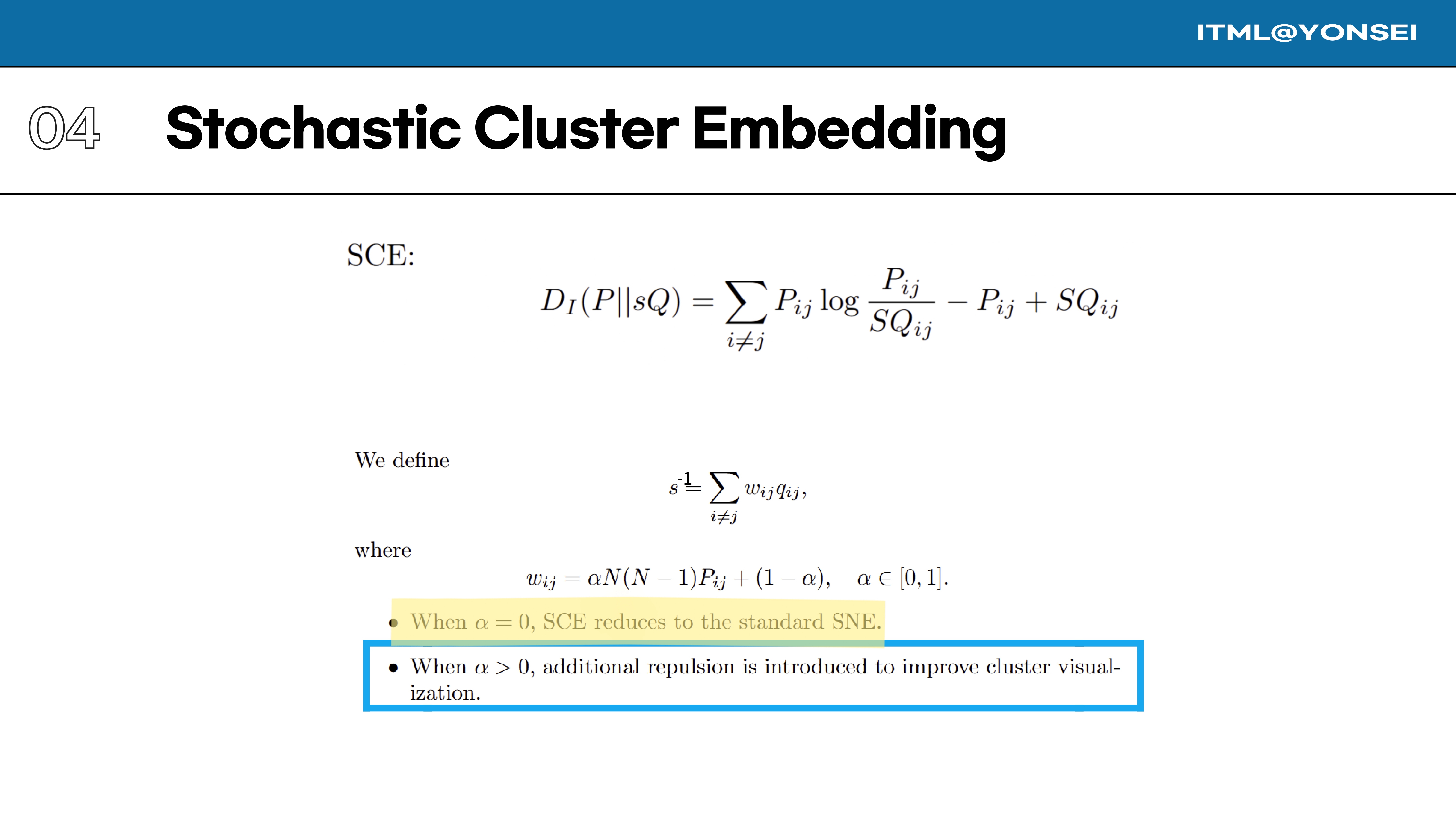
SCE defines the scaling factor ’s’ using a weighted sum controlled by the parameter α, which introduces additional repulsion to improve cluster quality. A key methodological point, raised by Reviewer C43T, was why ’s’ is treated as a constant during optimization when it is a function of the embeddings. The authors clarified that they use an interleaving optimization strategy: the model parameters are optimized while ’s’ is fixed, and then ’s’ is periodically updated based on the new embeddings.

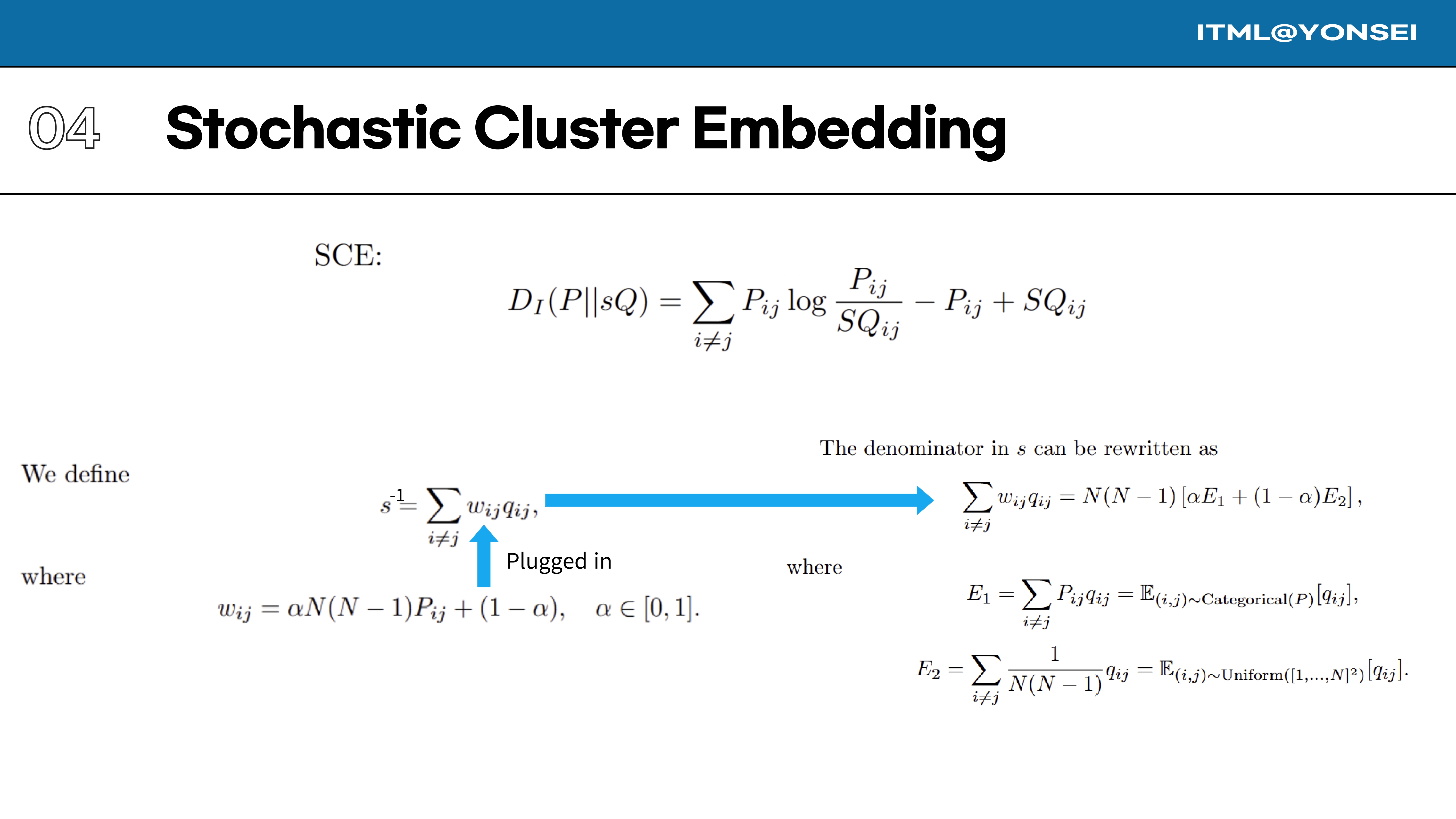
By plugging this definition of the weights $w_{ij}$ into the formula for ’s’, the denominator term can be rewritten as a sum of two expectations.

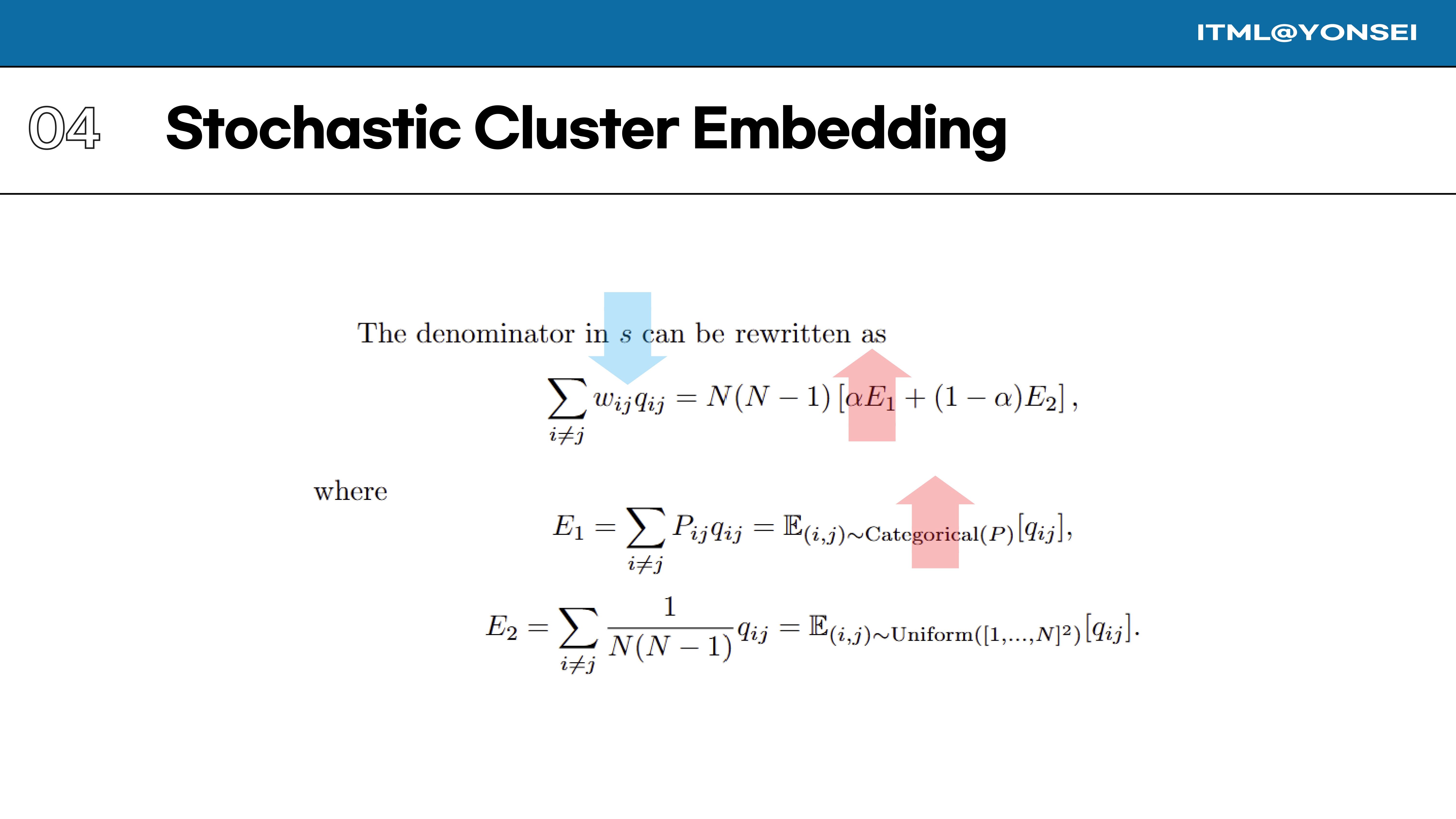
These two expectations have clear interpretations: $E_1$ is the expected similarity for pairs drawn from the target distribution P, while $E_2$ is the expected similarity for pairs drawn uniformly at random from all possible pairs.

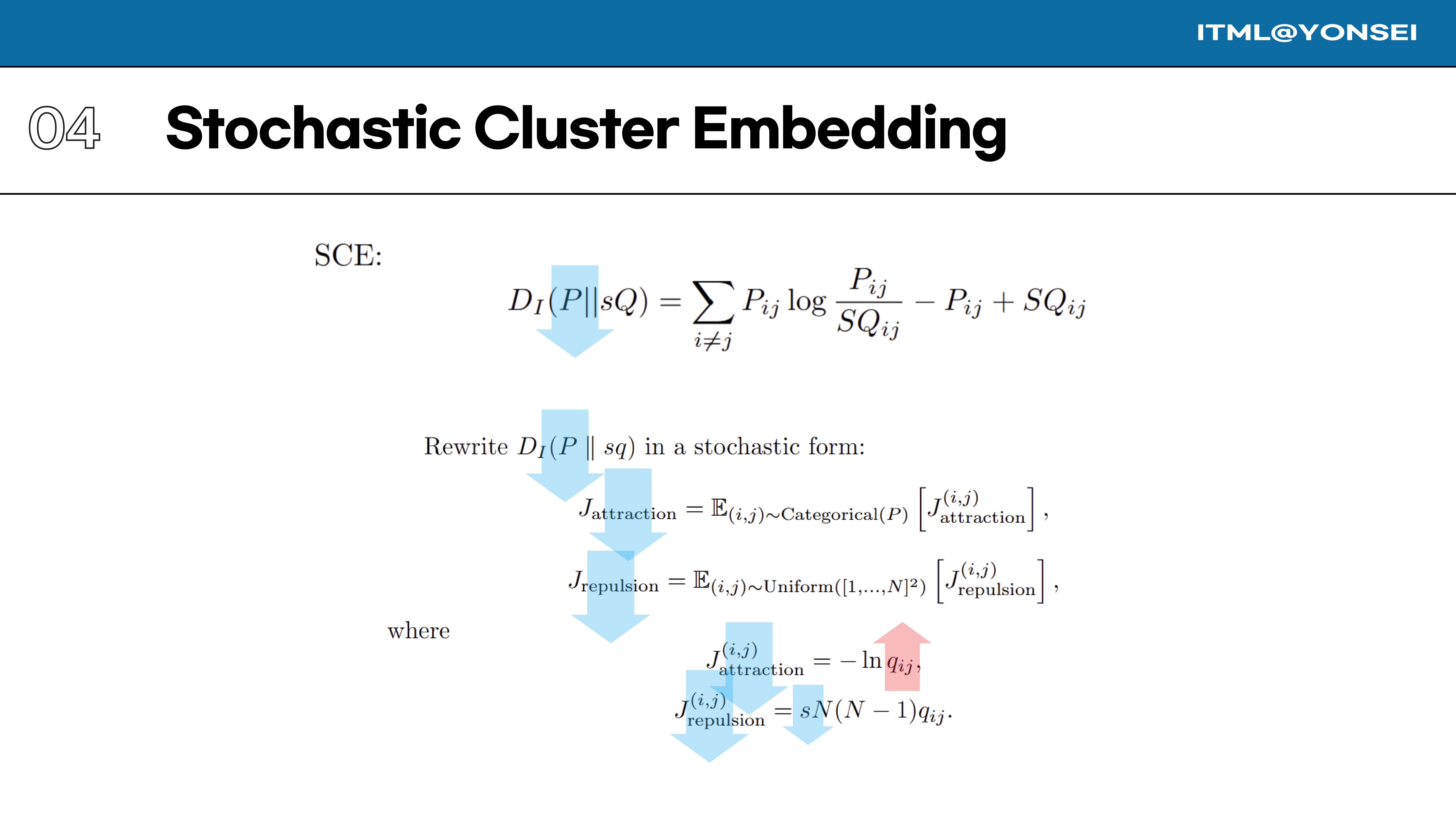
This formulation allows the I-divergence objective to be rewritten in a stochastic form, separating it into an attraction term based on the target distribution and a repulsion term based on the uniform distribution. The terms themselves are simple functions of the similarity $q_{ij}$.

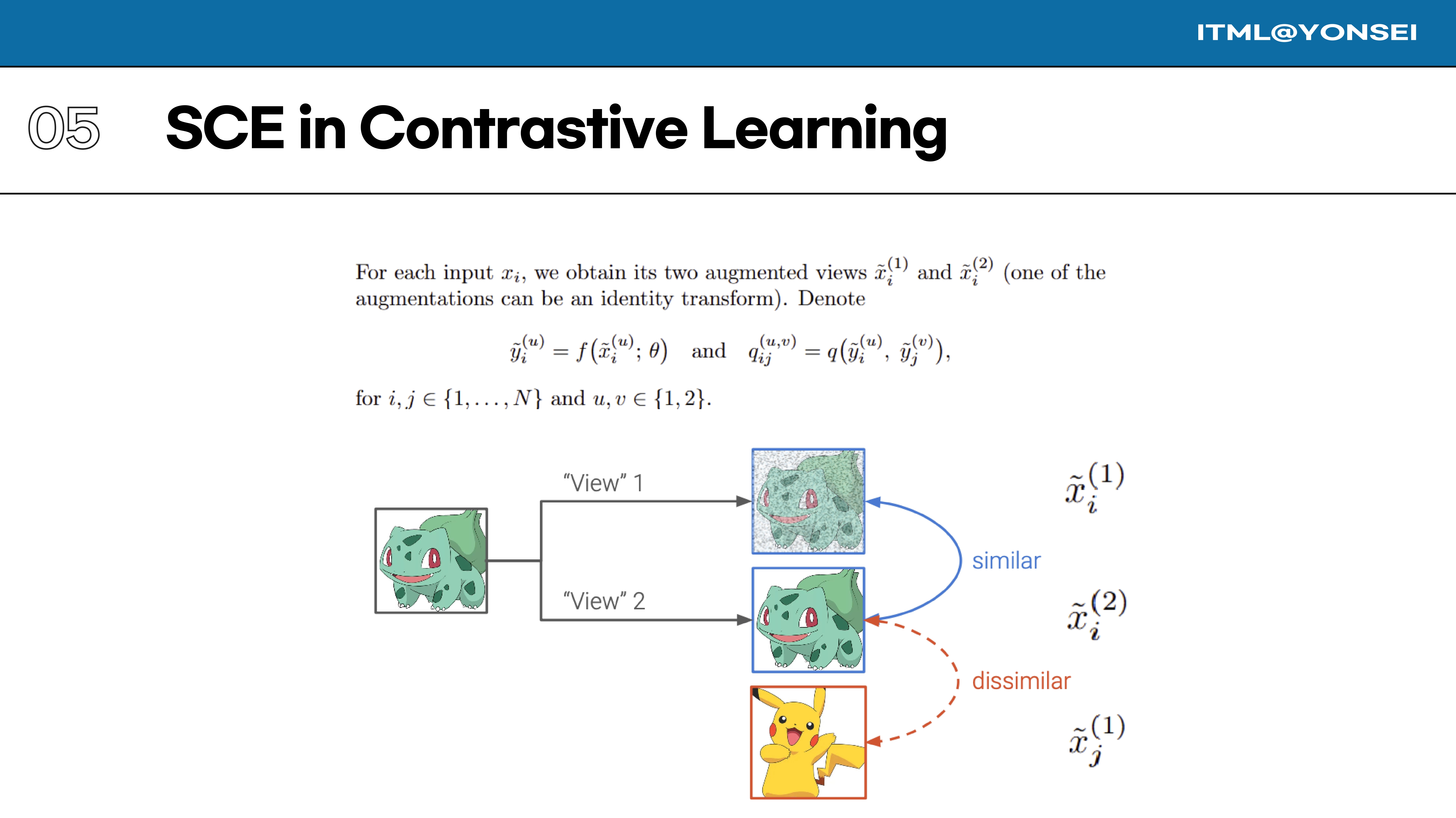
Now, let’s apply this SCE framework to Contrastive Learning. In our setting, for each input $x_i$, we generate two augmented views, $\tilde{x}{i}^{(1)}$ and $\tilde{x}{i}^{(2)}$. We denote their embeddings as $\tilde{y}{i}^{(u)}$ and the similarity between any two embeddings as $q{ij}^{(u,v)}$.

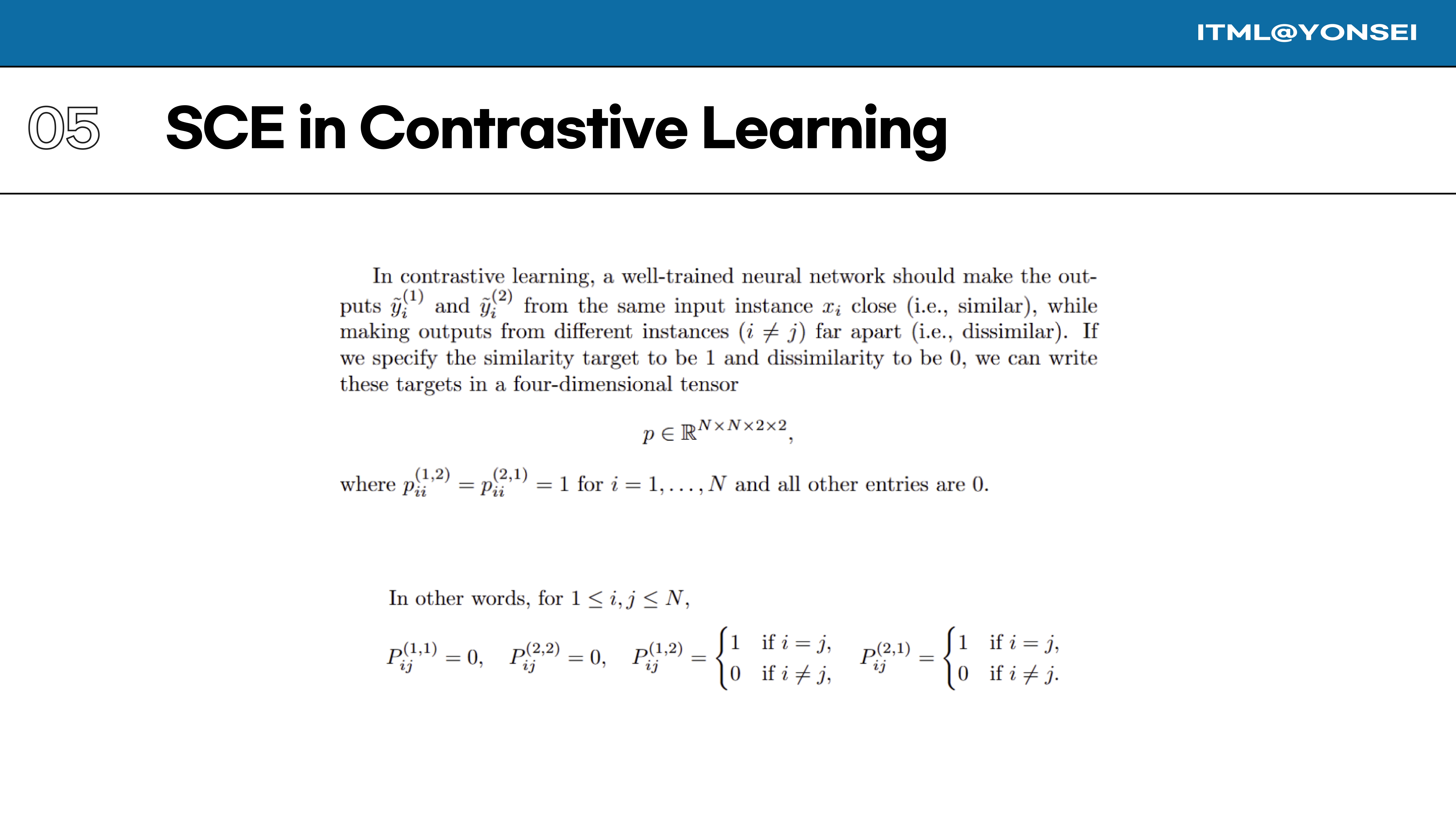
The goal in contrastive learning is to make embeddings from the same instance ($i=j$) similar, and embeddings from different instances ($i \ne j$) dissimilar. We can formally define this as a target tensor $p$, where the target similarity is 1 only for positive pairs ($p_{ii}^{(1,2)}$ and $p_{ii}^{(2,1)}$) and 0 for all other pairs.

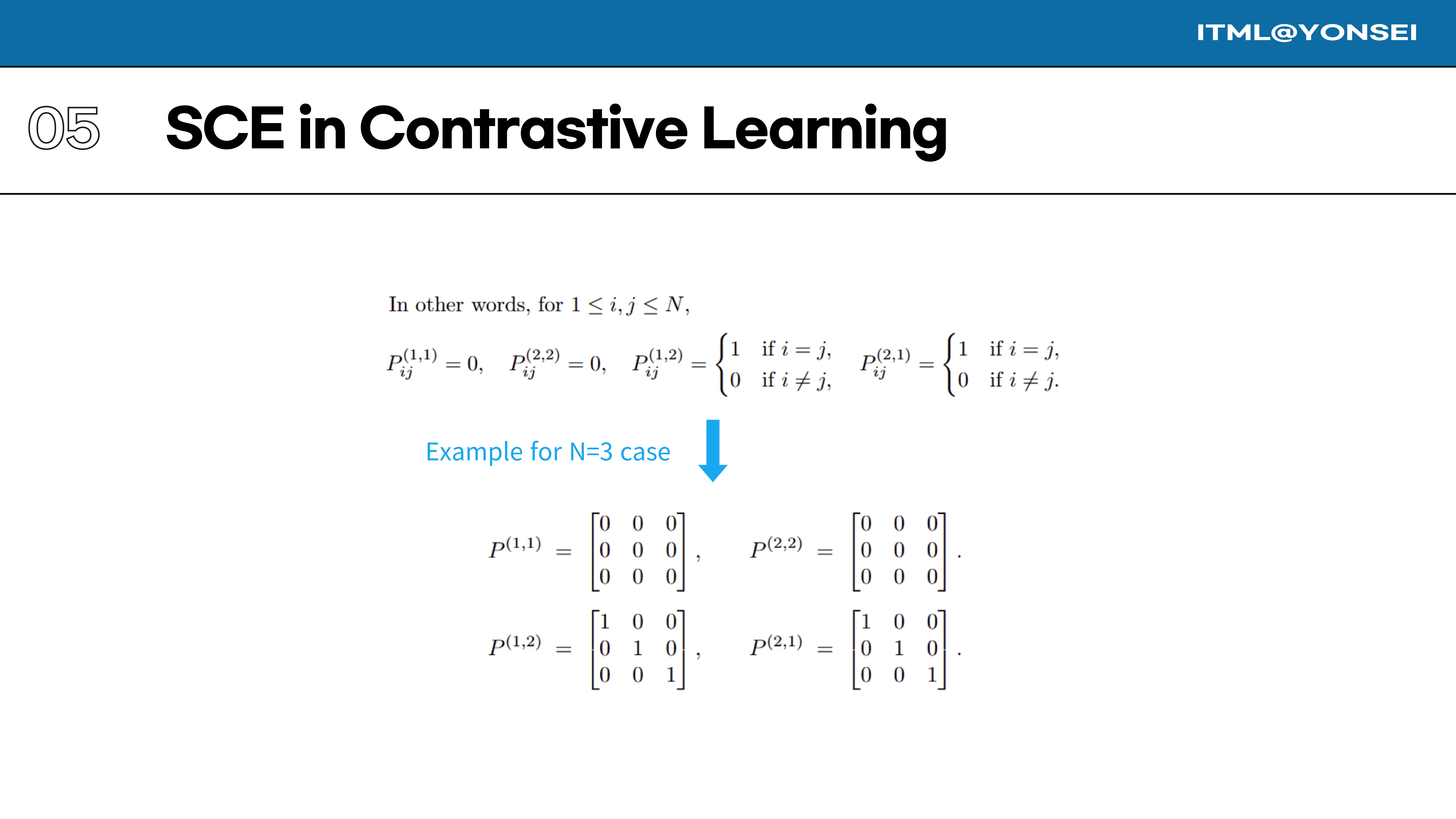
This slide provides a concrete example of the target tensor $P$ for a case with N=3 instances. The matrices for same-view similarities ($P^{(1,1)}, P^{(2,2)}$) are all zeros, while the matrices for cross-view similarities ($P^{(1,2)}, P^{(2,1)}$) are identity matrices, capturing the positive pair targets.

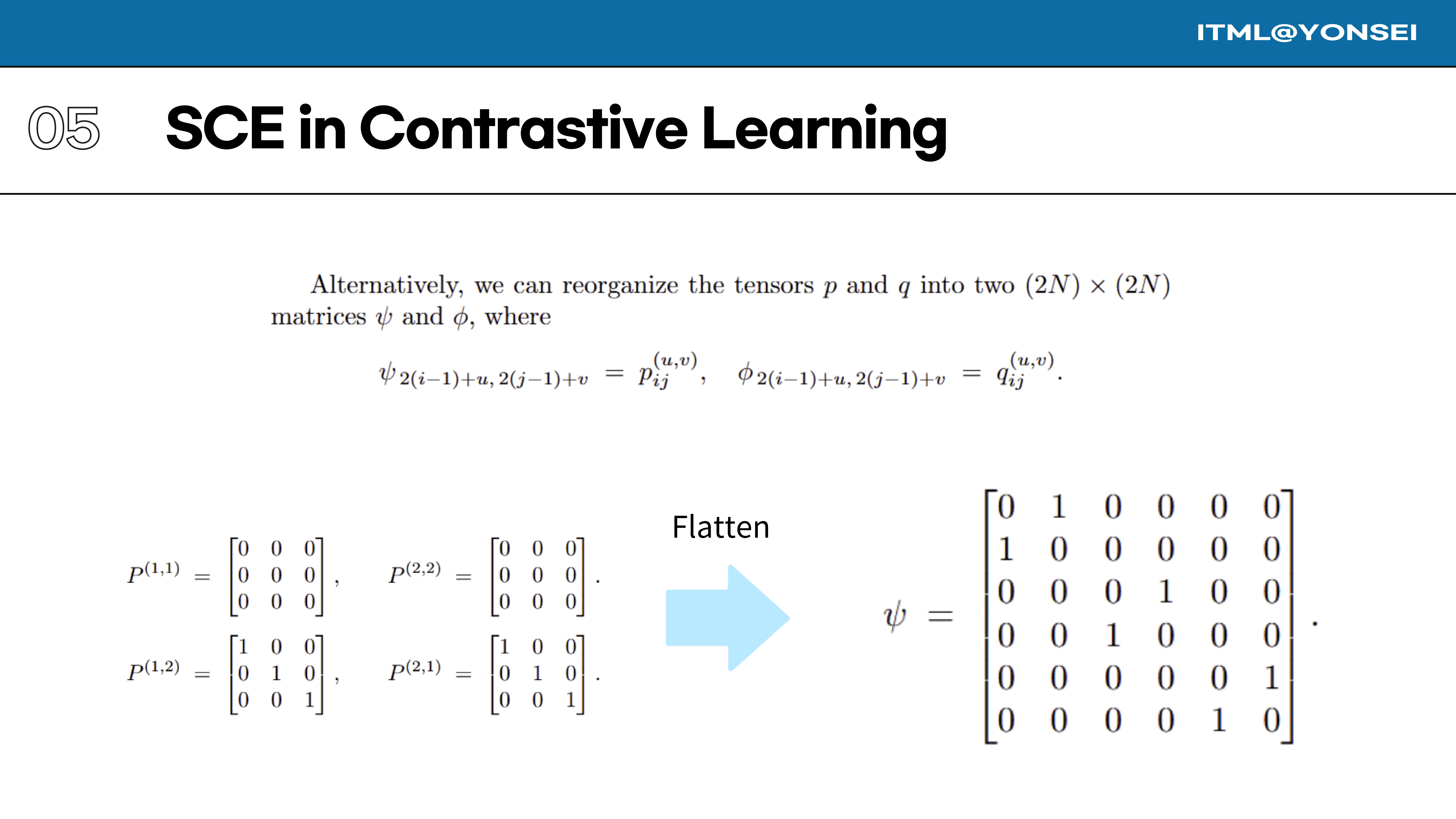
To simplify the math, we can flatten this four-dimensional tensor structure into standard 2D matrices. The $2N \times 2N$ target matrix $\psi$ is formed by reorganizing the elements of the tensor $p$. This results in a sparse matrix where the identity matrices from the tensor become off-diagonal blocks.

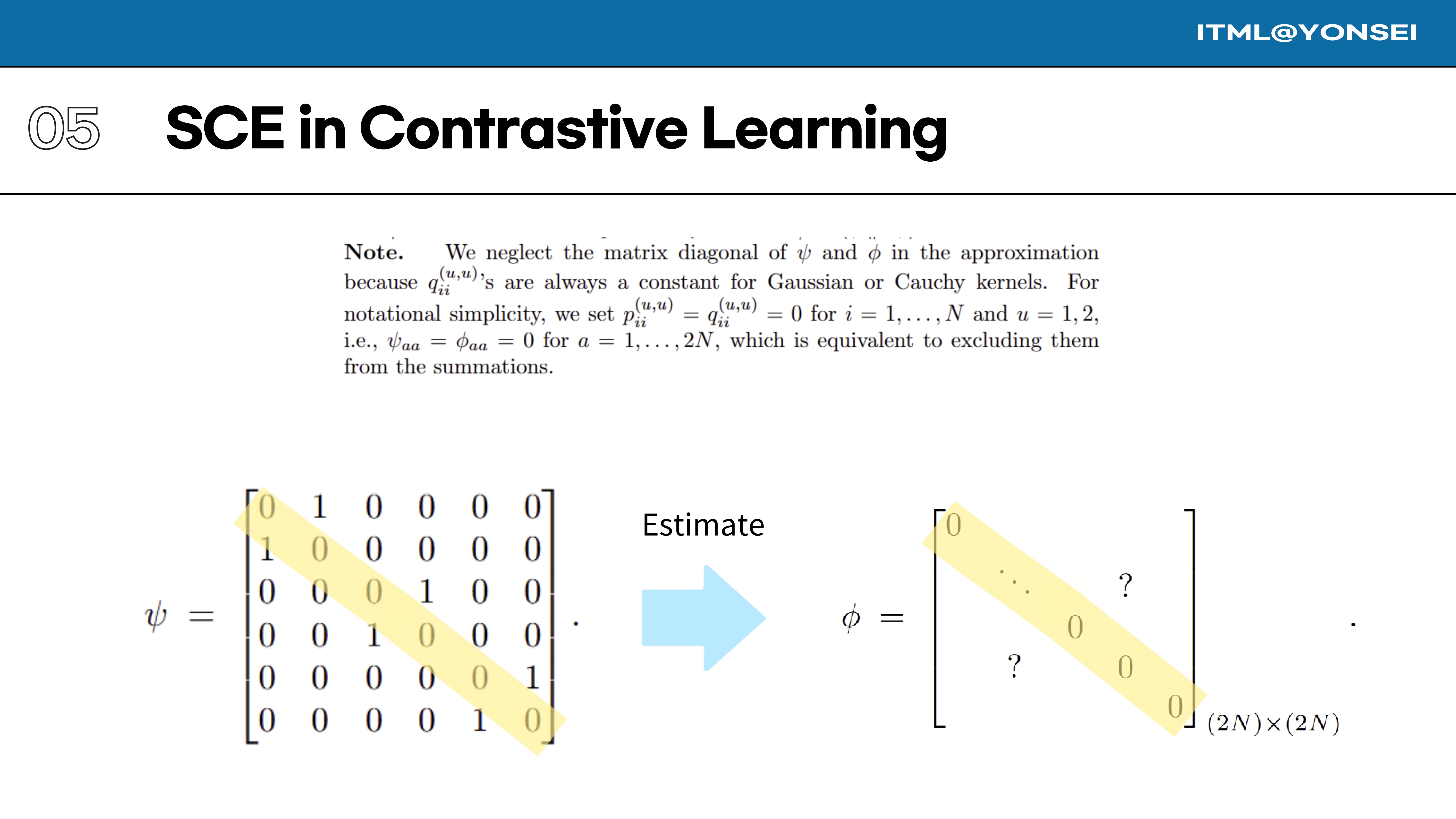
For notational simplicity, we neglect the diagonal elements of the matrices $\psi$ and $\phi$ in the approximation, as they are constant for the kernels used and do not affect the optimization.

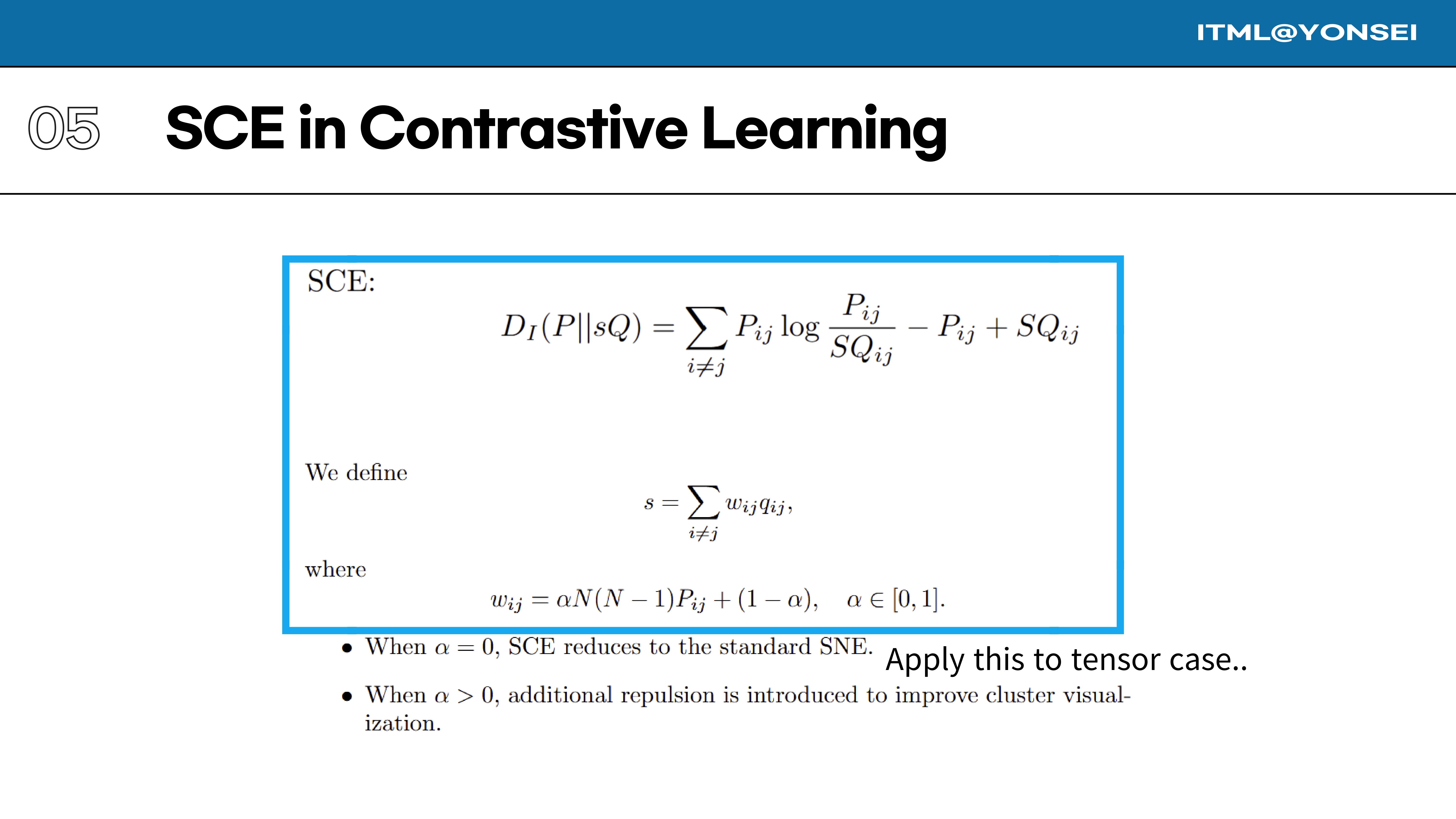
Now we apply the SCE I-divergence formula, but to our new flattened matrices $\psi$ and $\phi$ which represent the contrastive learning problem.

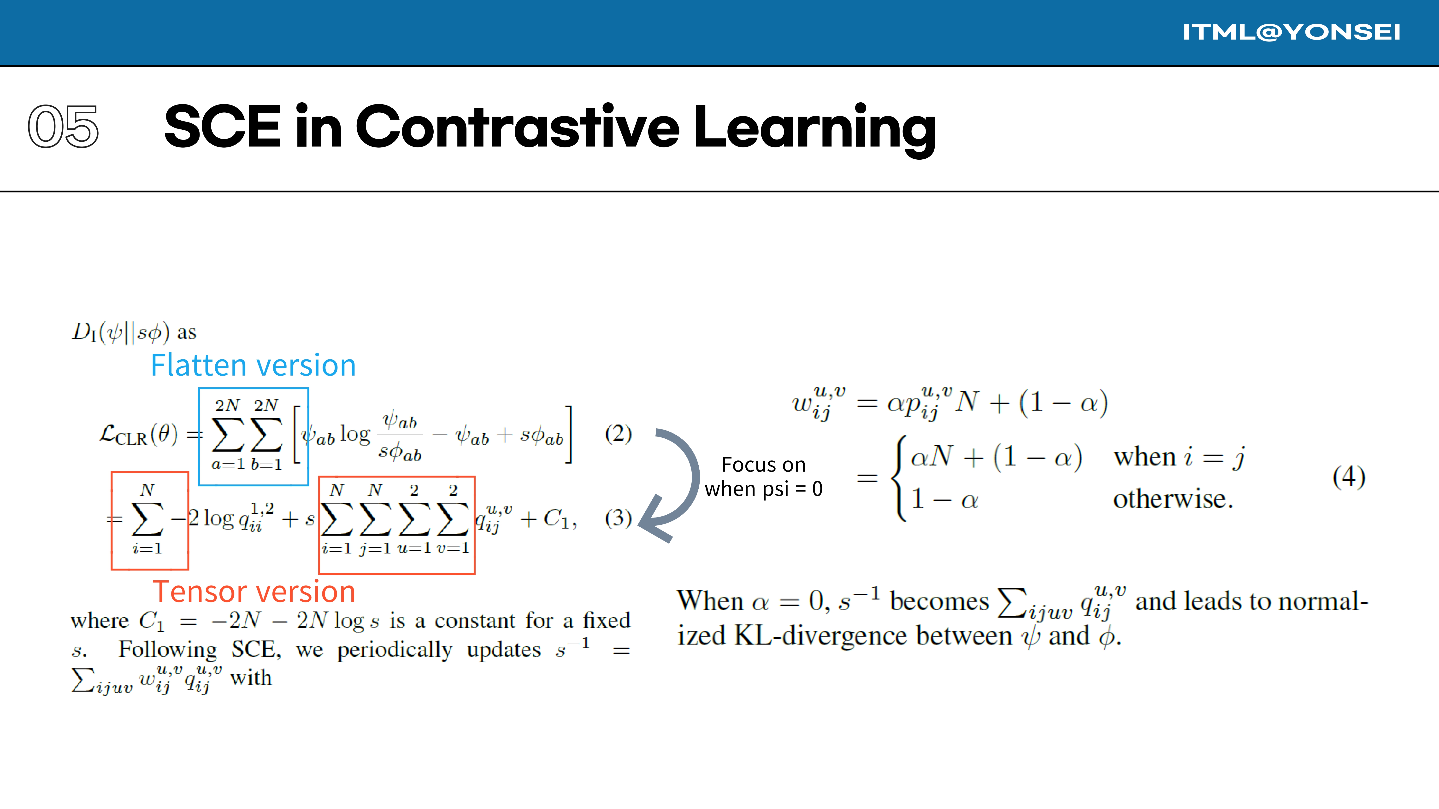
Applying the I-divergence $D_{I}(\psi||s\phi)$ and using the specific structure of our target matrix $\psi$ (which is mostly zeros), the loss function simplifies significantly. The scaling factor $s$ is updated periodically, with its weights $w_{ij}^{u,v}$ also adapted for the contrastive case.

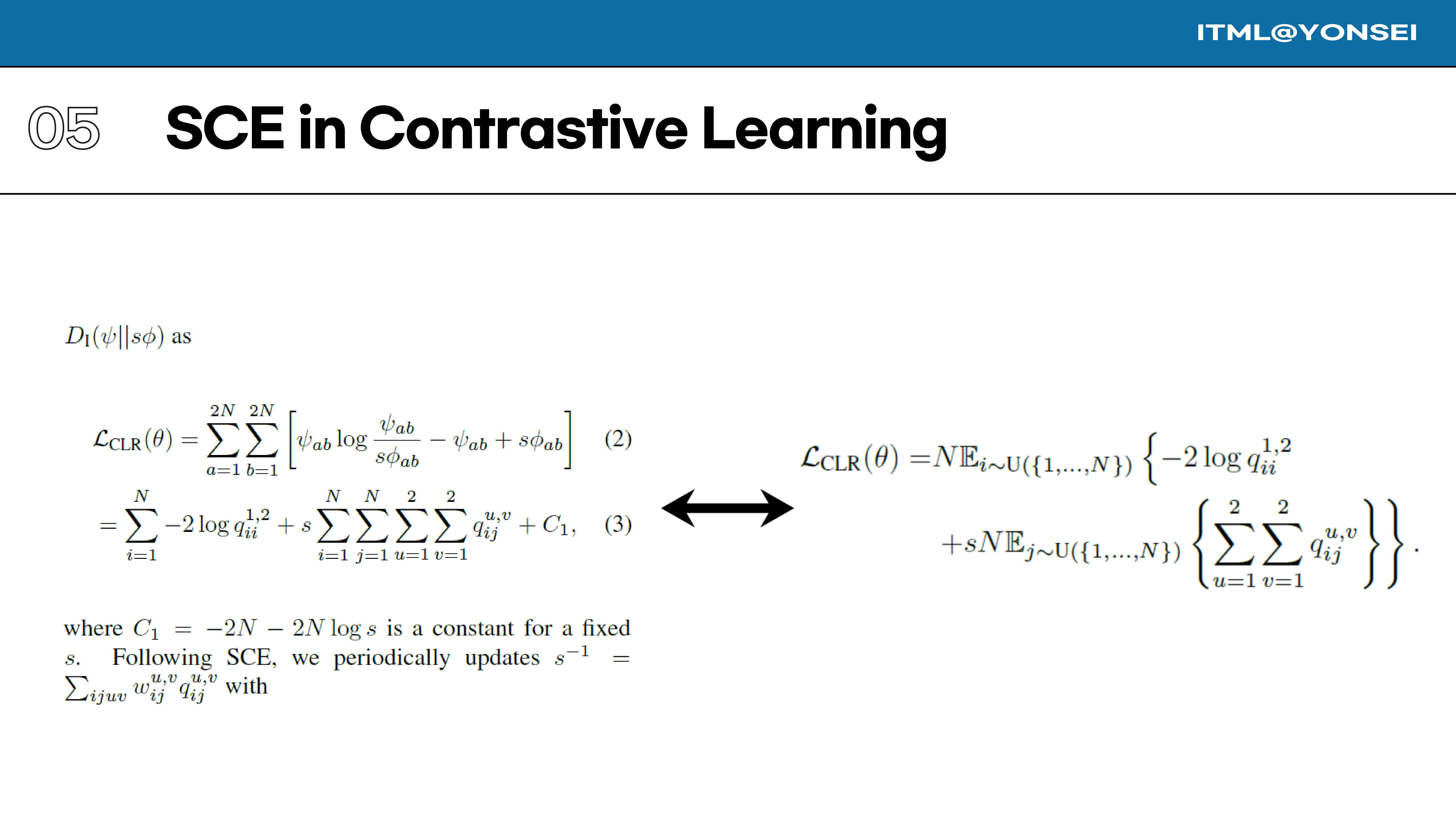
The full loss function $\mathcal{L}{CLR}(\theta)$ can be expressed as an expectation over the data indices. This form consists of a term for positive pairs ($log~q{ii}^{1,2}$) and a repulsion term involving a sum of similarities over all pairs.

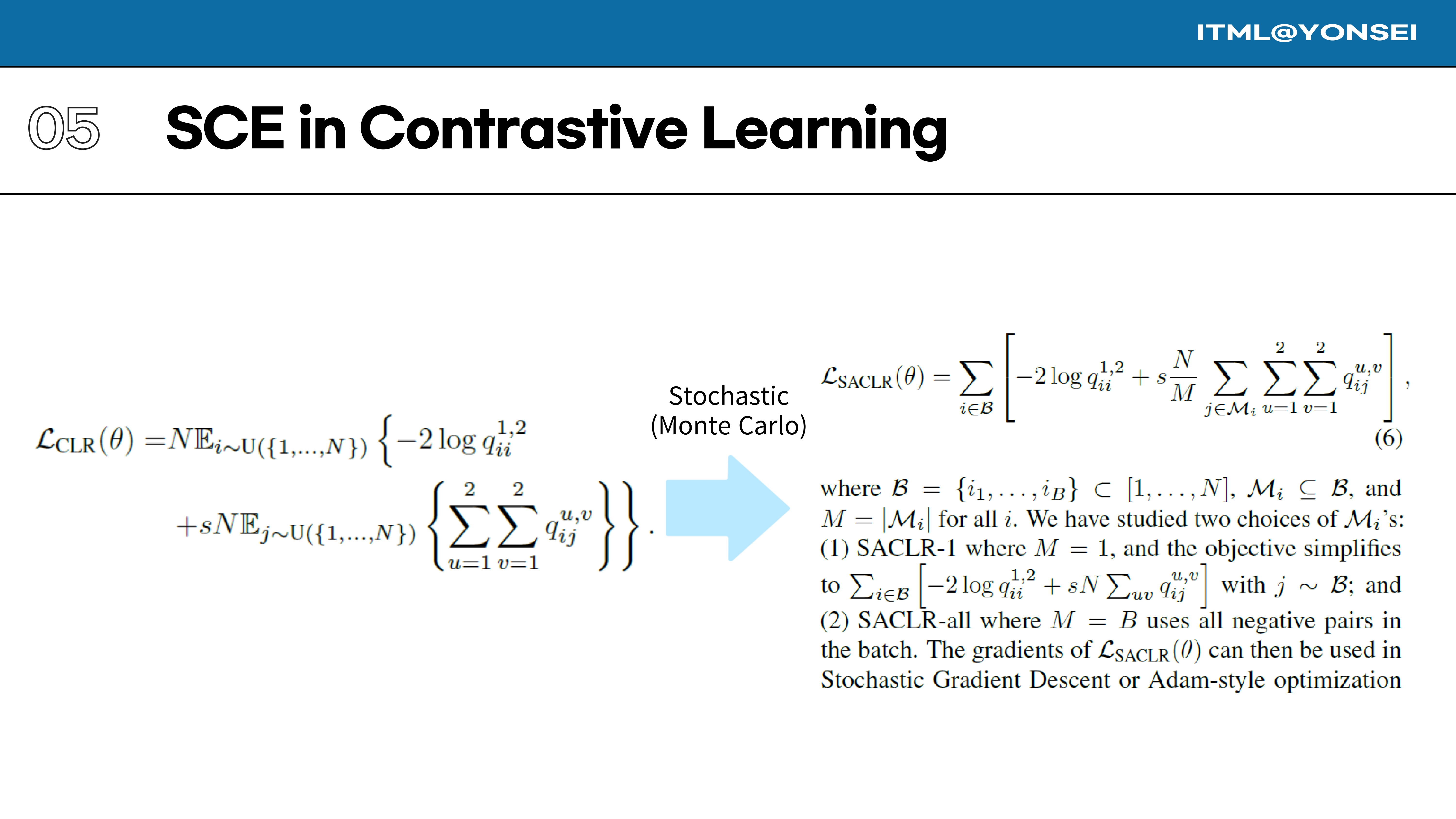
To make this computationally feasible, we use a Monte Carlo approximation. This gives us the final SACLR objective, $\mathcal{L}{SACLR}(\theta)$, which is calculated over a mini-batch $\mathcal{B}$ and a set of M negative samples $\mathcal{M}{i}$. The paper studies two variants: SACLR-1 (M=1) and SACLR-all (M=B).

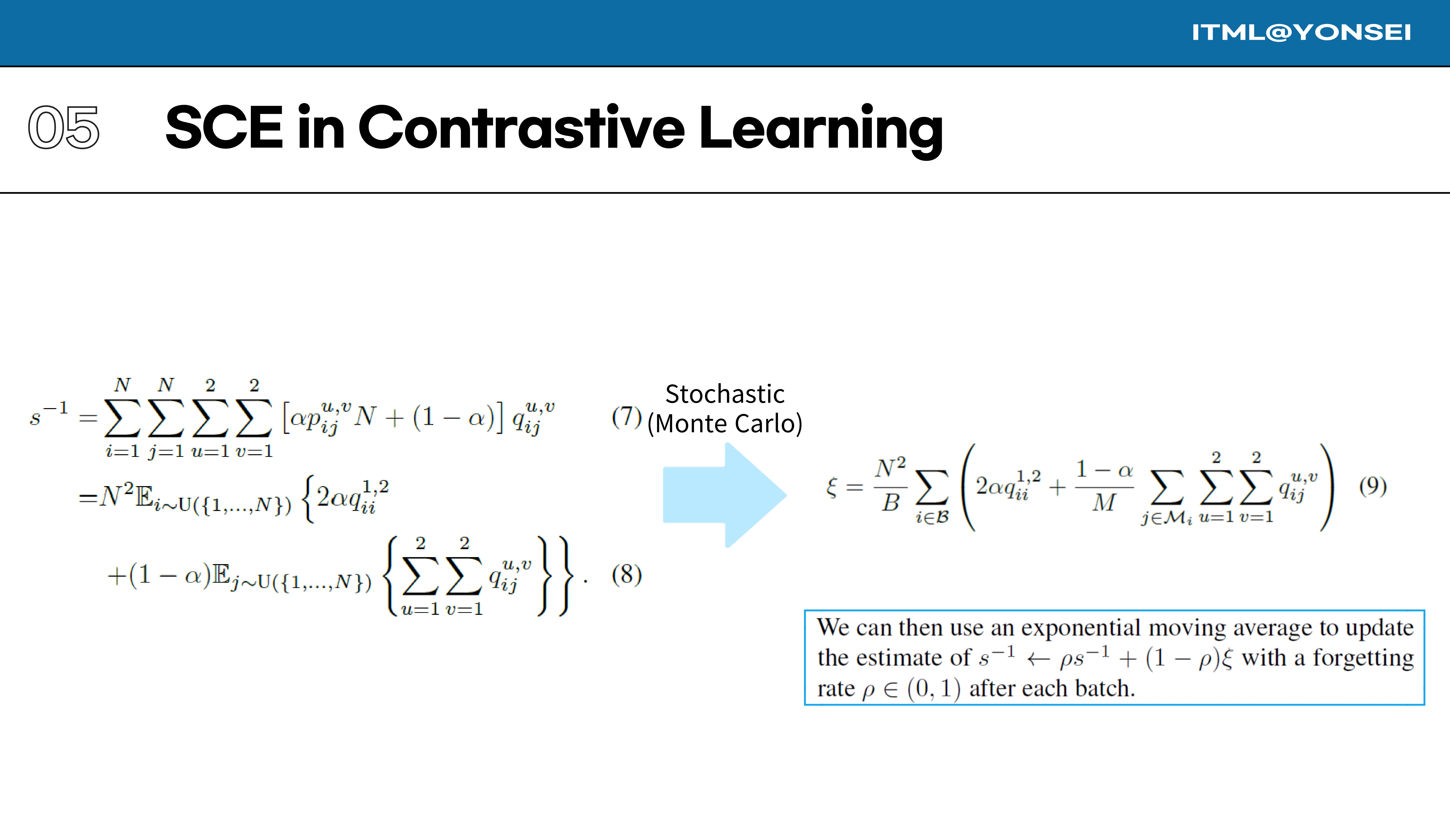
The scaling factor $s$ is also estimated stochastically. Its inverse, $s^{-1}$, is approximated using samples from the mini-batch, and this estimate is updated smoothly using an exponential moving average (EMA) after each batch.

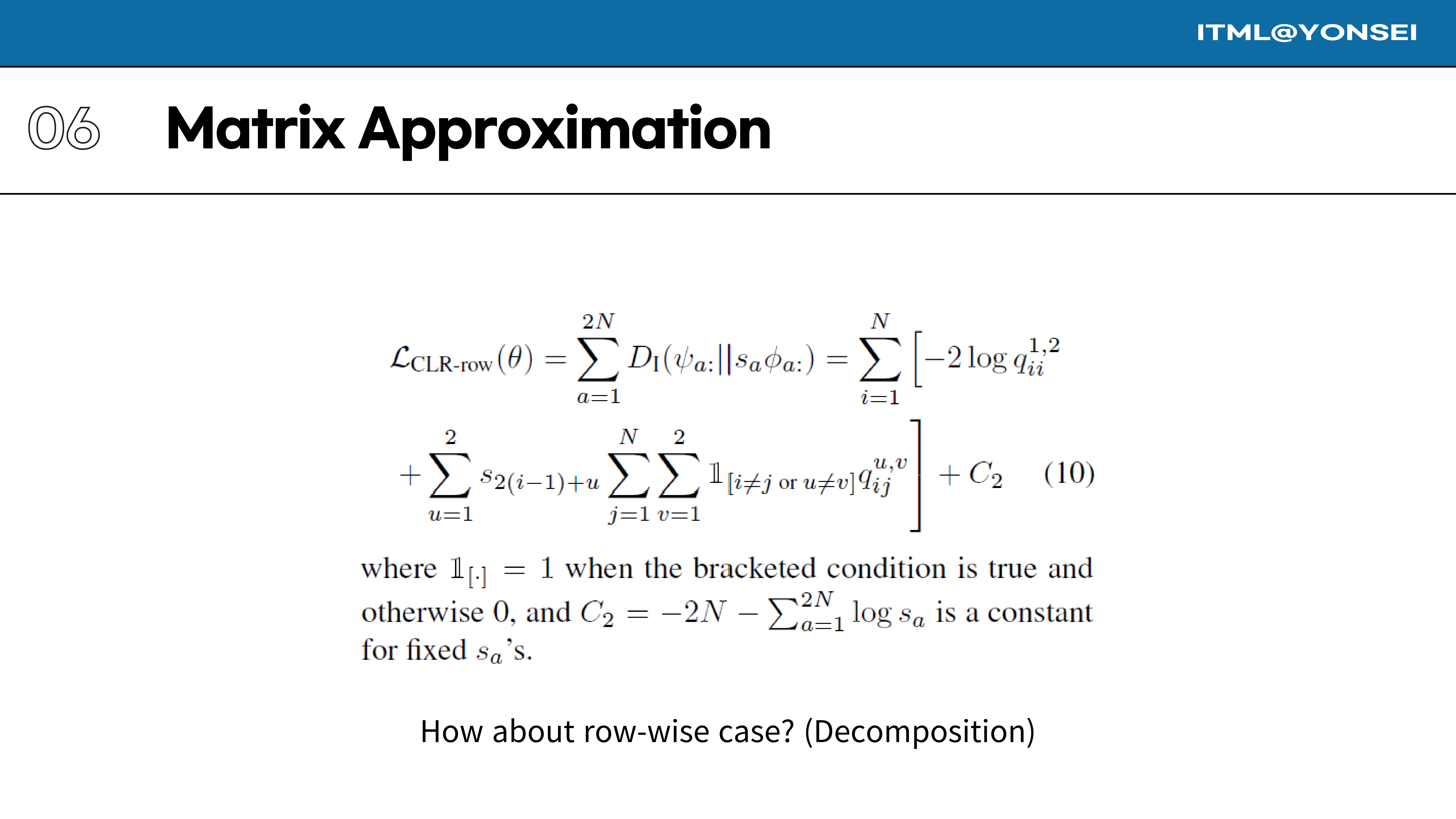
The paper also explores a row-wise decomposition of the matrix approximation. Instead of one global scaling factor ’s’, each row ‘a’ of the similarity matrix gets its own scaling factor $s_a$. This results in the loss function $\mathcal{L}_{CLR-row}(\theta)$.

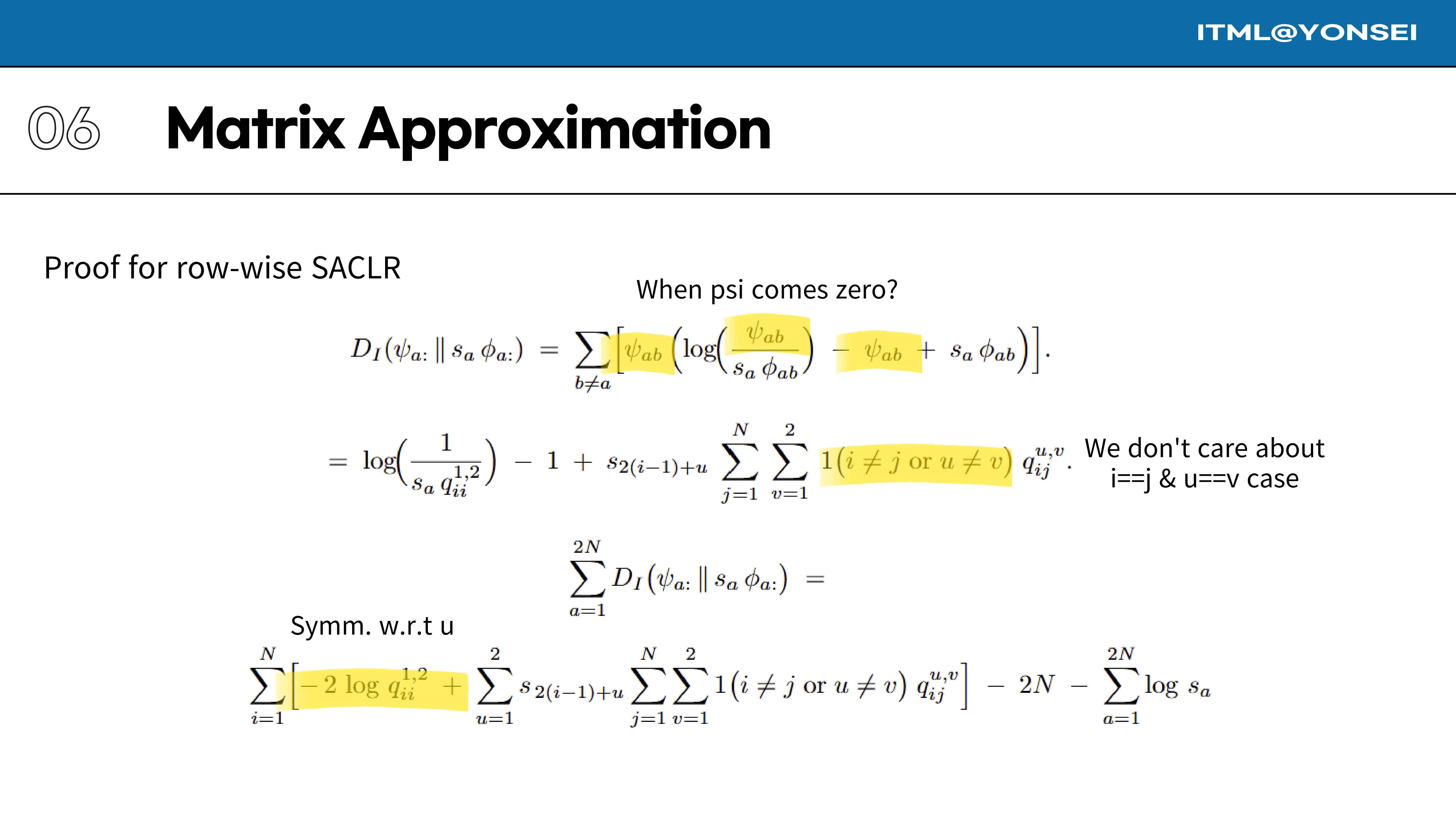
This slide provides proof for the simplified row-wise SACLR loss function. By substituting the sparse target matrix $\psi$ into the general I-divergence formula and summing over all rows, we arrive at the expression shown.

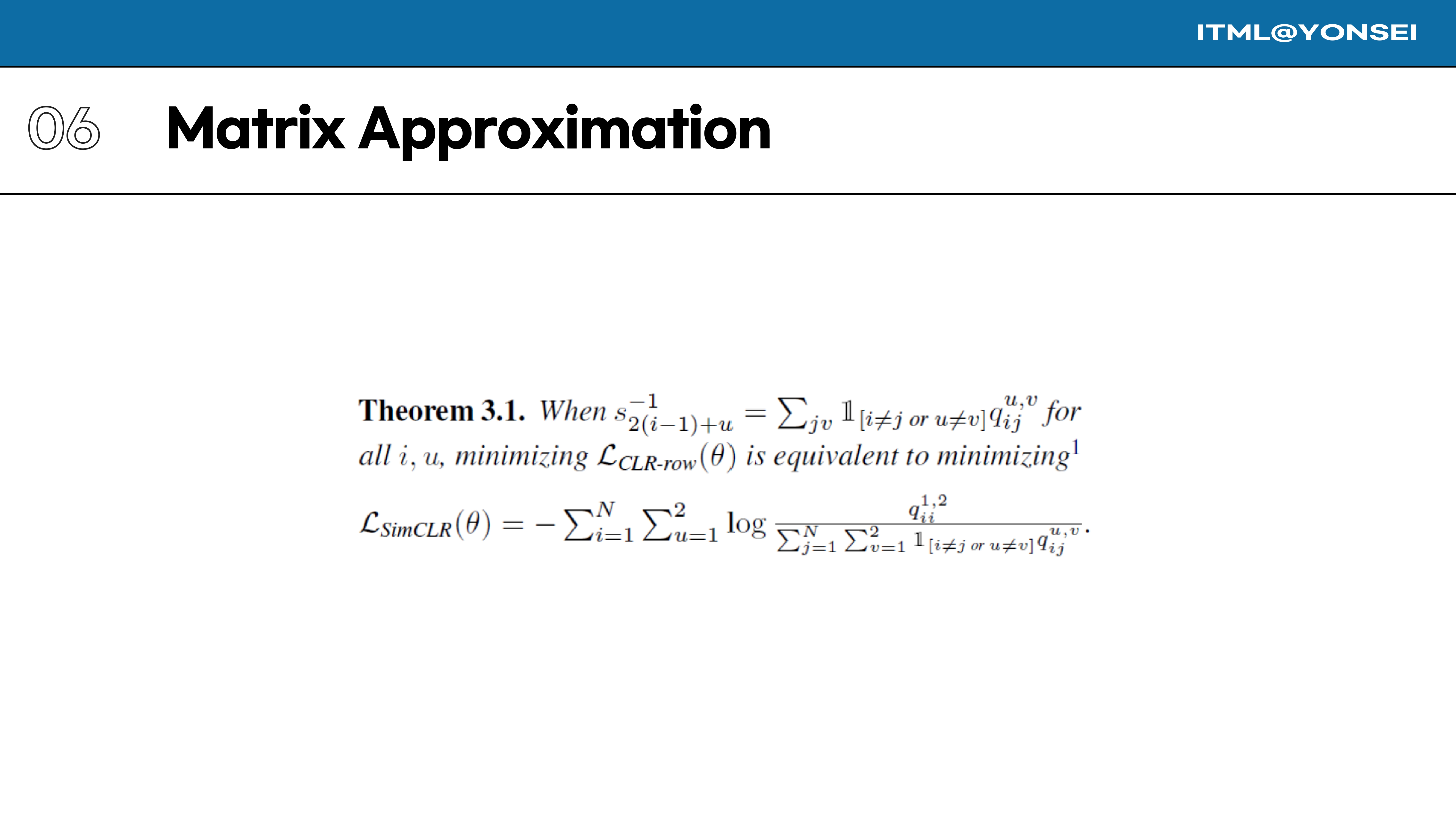
A key theoretical finding presented in the paper is that under specific conditions, the SACLR-row objective becomes equivalent to the SimCLR loss. This link, however, became a point of discussion during the review. Reviewer gz9D argued that this equivalence doesn’t explain why SACLR should be expected to outperform SimCLR. The authors countered that the method’s advantage comes not from this specific condition, but from using a different, more flexible weighting scheme for the scaling factor.

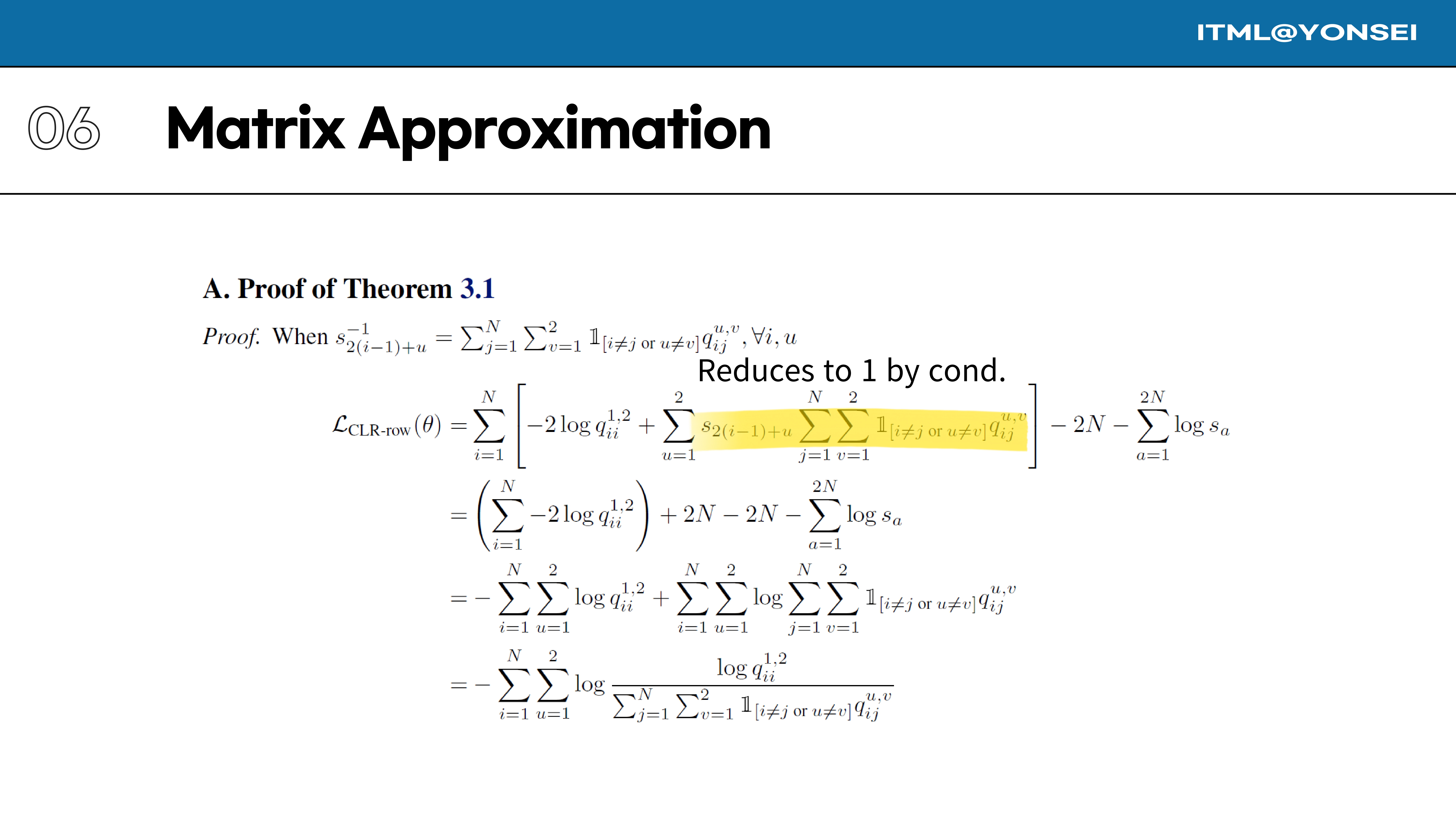
Here is the proof of Theorem 3.1. By substituting the condition for the scaling factors into the loss function, the repulsion term simplifies to a constant, and the remaining terms can be rearranged to form precisely the SimCLR objective.

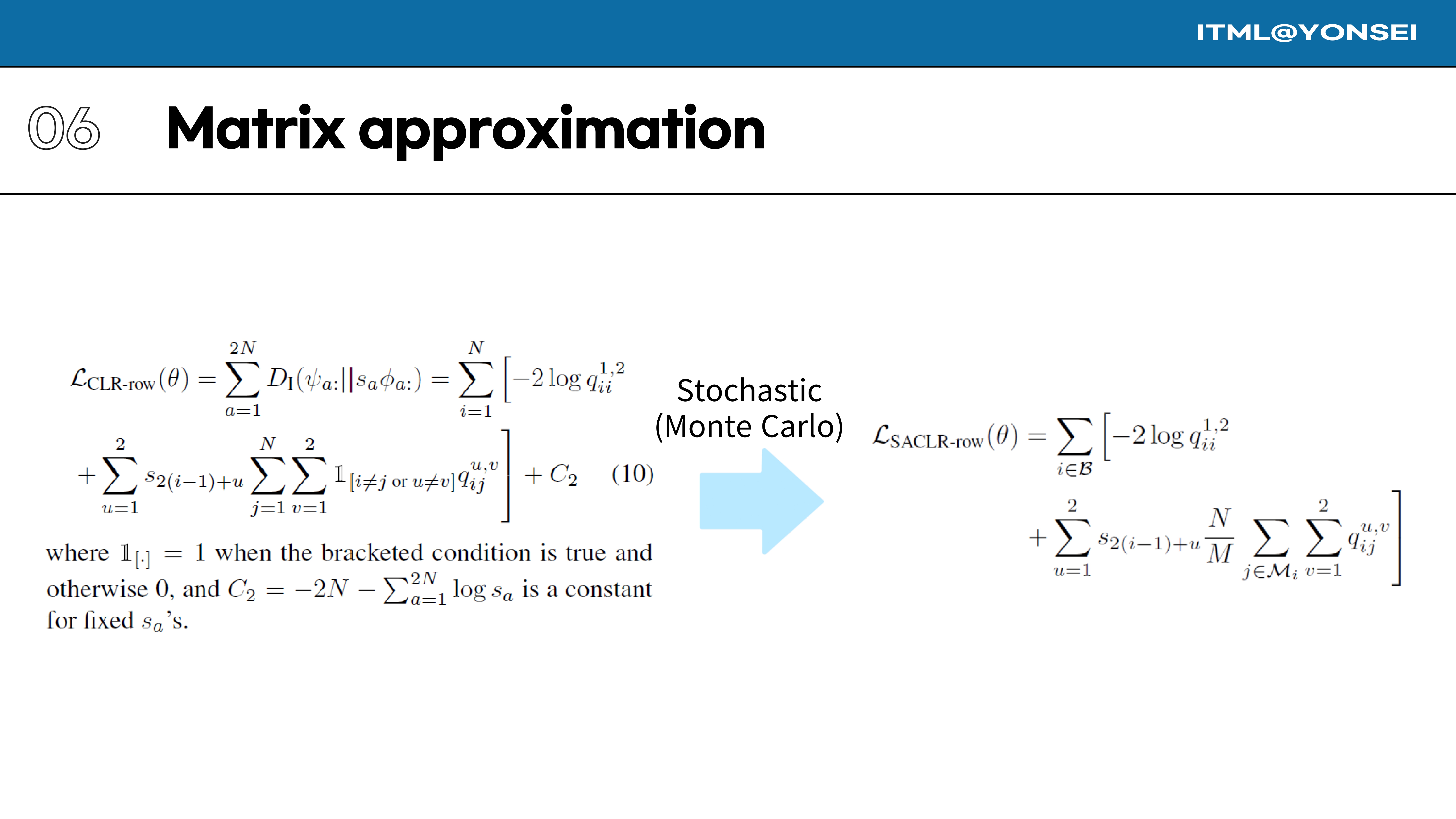
Just as with the full matrix version, the row-wise loss can be approximated stochastically for mini-batch training. This gives us the $\mathcal{L}_{SACLR-row}(\theta)$ objective.

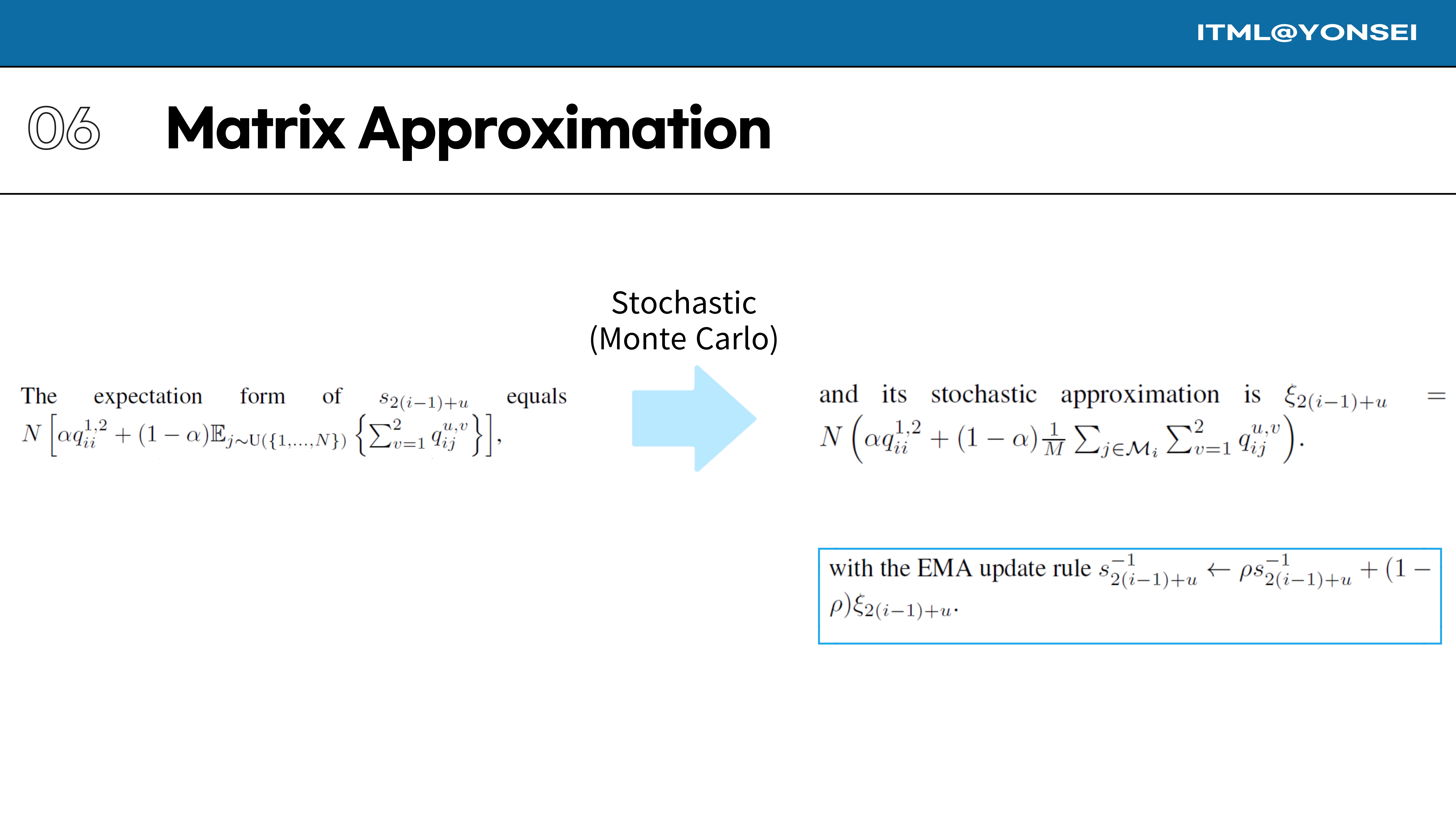
Similarly, the row-wise scaling factors $s_{2(i-1)+u}$ are estimated stochastically within each mini-batch and updated using an EMA rule.

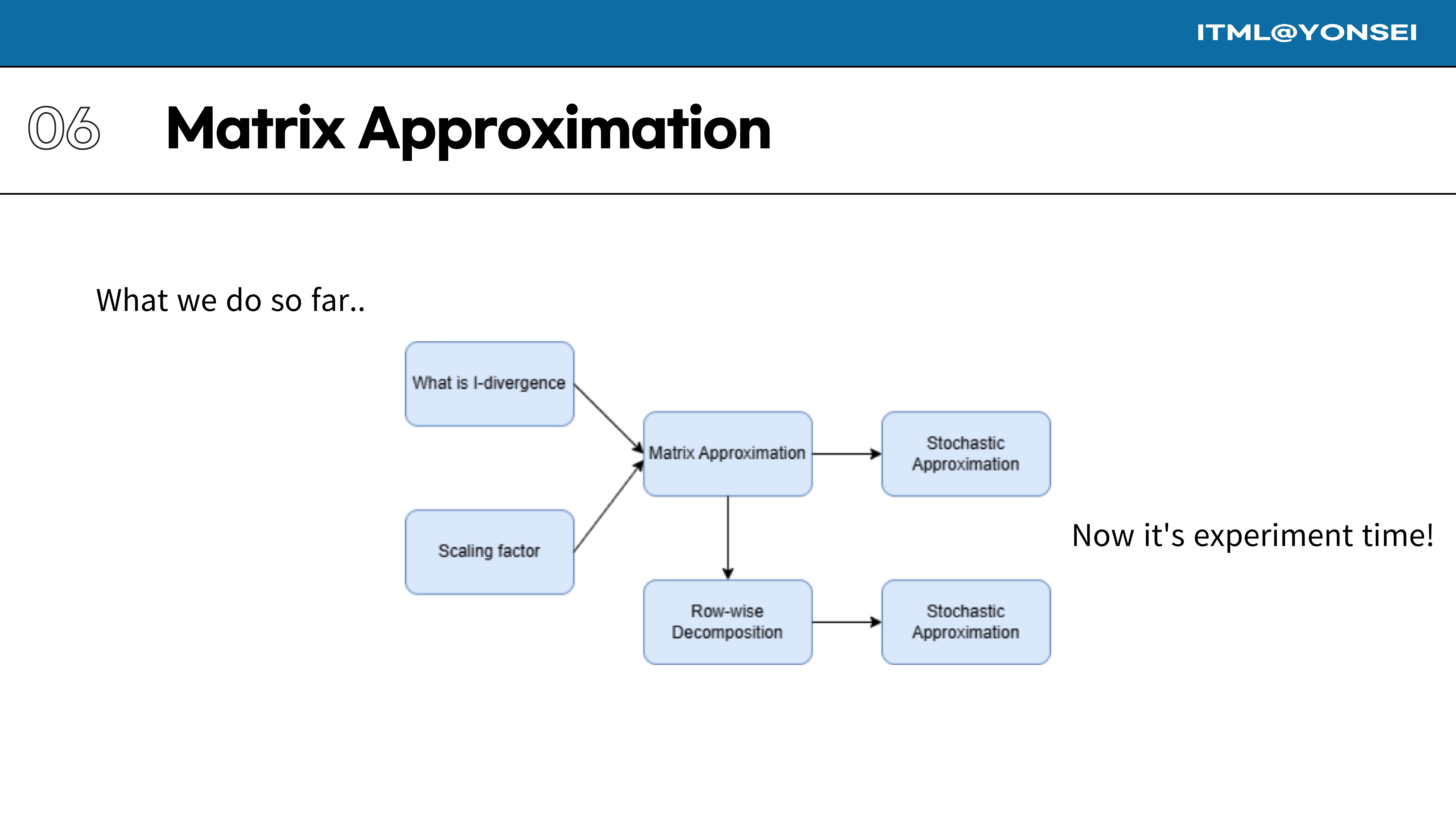
This diagram provides a summary of the theoretical framework I have just presented. We started with the concept of I-divergence and a scaling factor, which we used to build a matrix approximation. This was then decomposed row-wise, and both versions were made practical via stochastic approximation. Now, it’s time to see the experimental results.

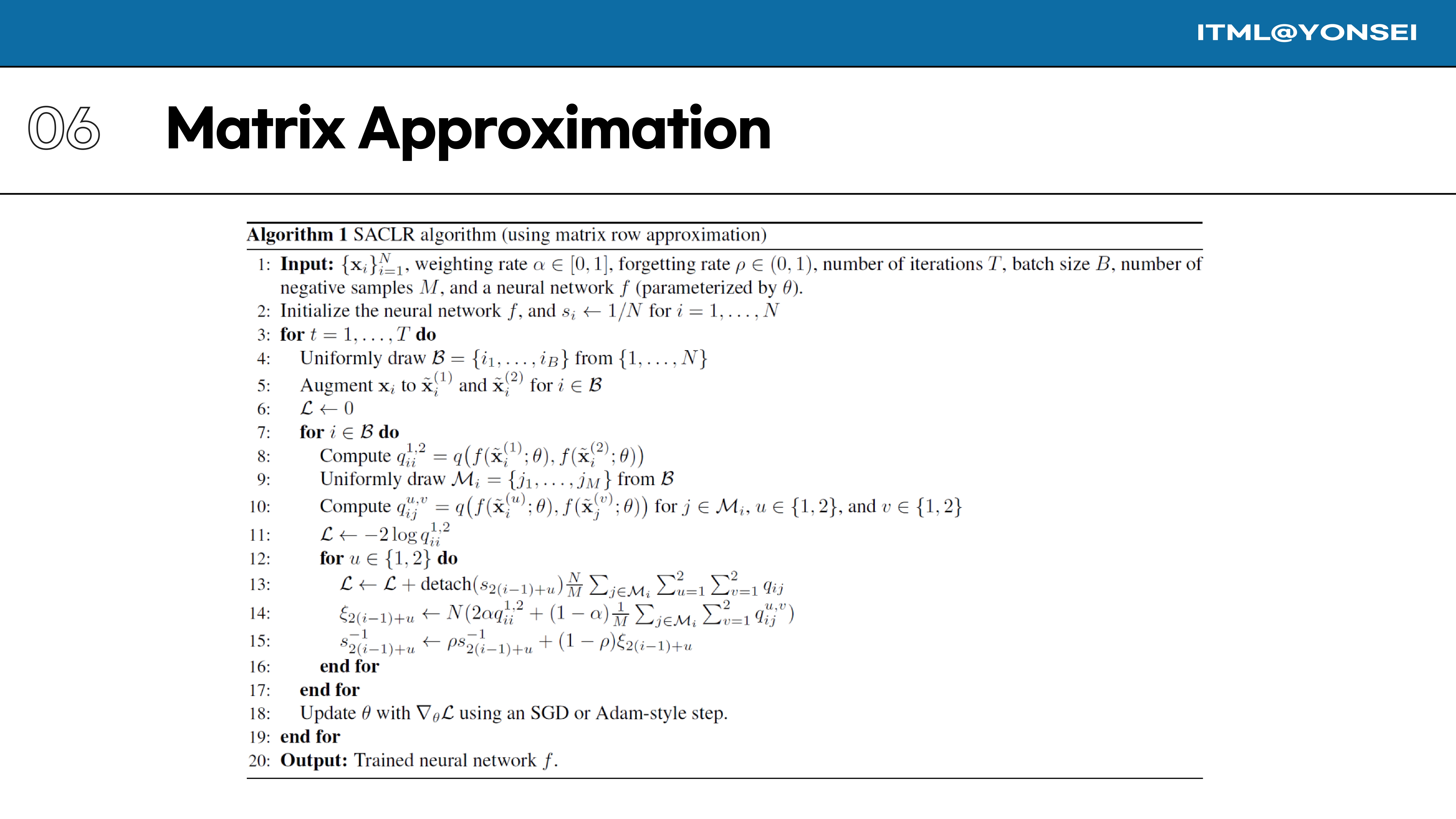
This slide presents the full pseudocode for the SACLR algorithm. A major point of contention in the initial review was that the paper claimed to be “more computationally efficient” without providing empirical data on runtime or memory. The detailed ablation studies on computational cost, shown later in the presentation, were added during the rebuttal period as a direct response to this criticism from the reviewers.

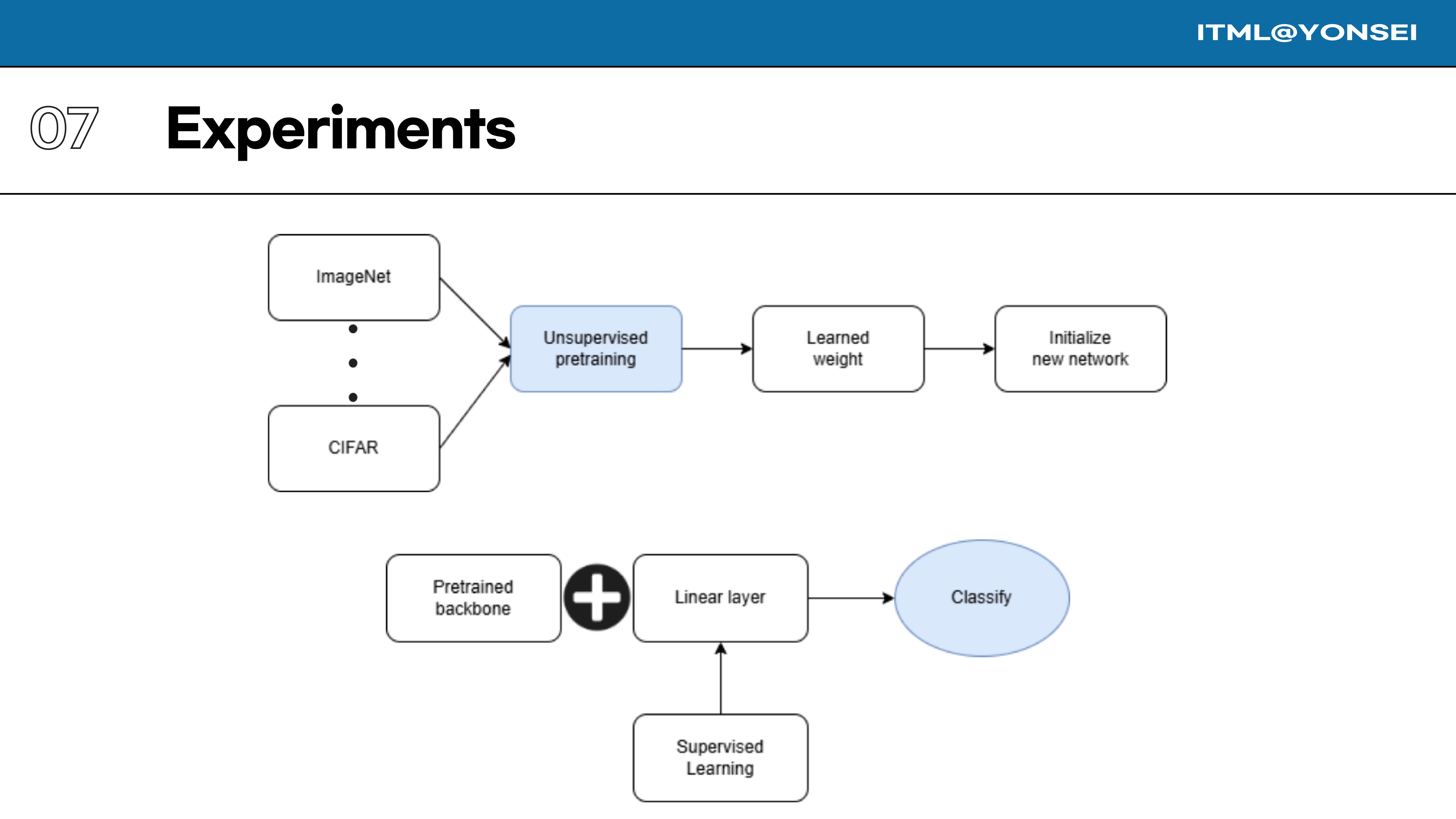
Now we move to the experiments section. The standard evaluation protocol for self-supervised methods is used: first, a model is pre-trained without labels on a dataset like ImageNet or CIFAR. The learned weights from this backbone are then used to initialize a new network, a linear layer is added, and this new network is trained with labels to perform a classification task.

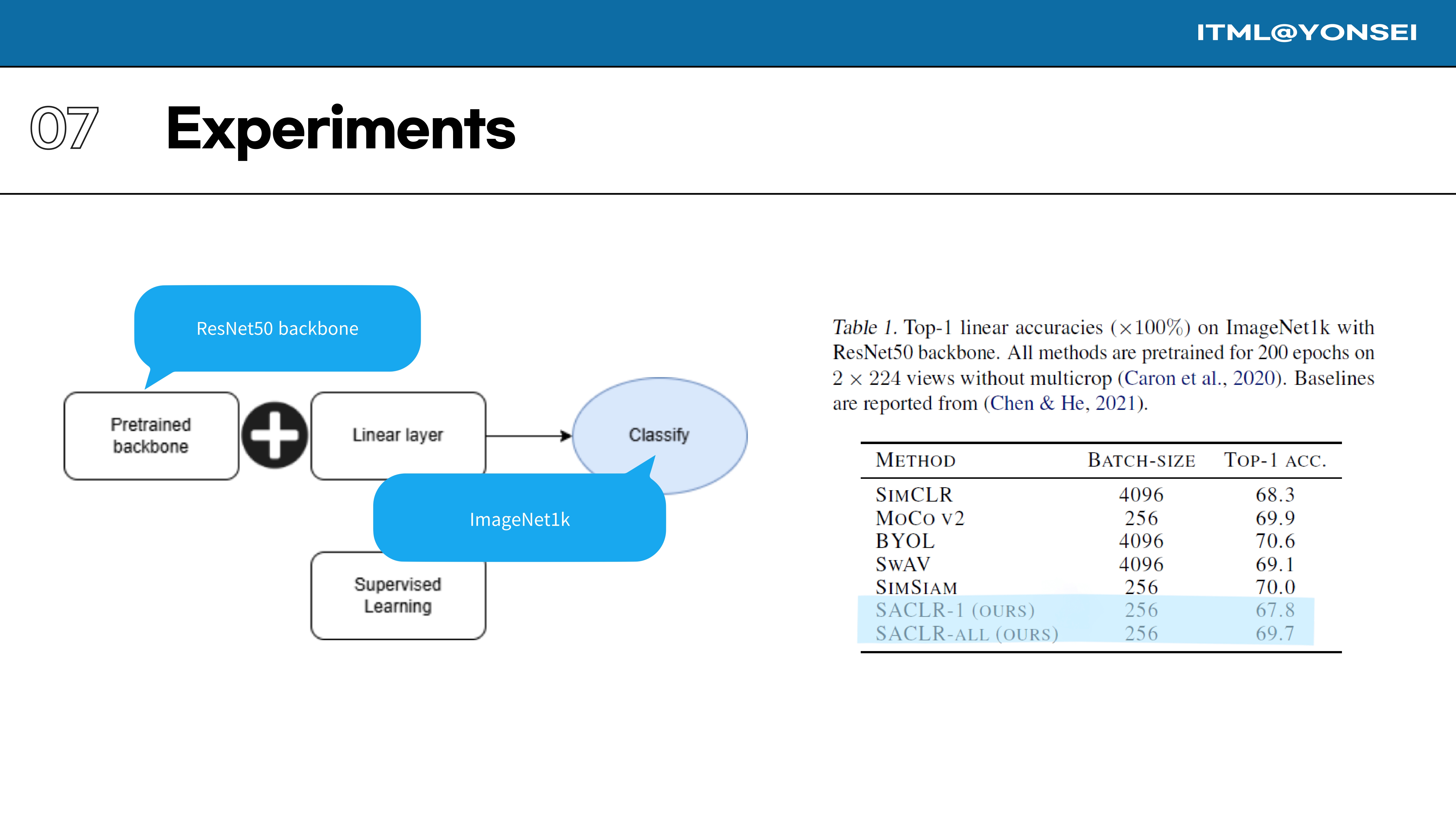
Table 1 shows the Top-1 linear classification accuracies on ImageNet. While SACLR-ALL is shown to be competitive with some methods like MoCo v2, this comparison drew significant criticism during the review process. The Area Chair and multiple reviewers stated that the baseline methods used for comparison were “weak” and the performance gains “marginal,” noting that many stronger, more recent methods were omitted.

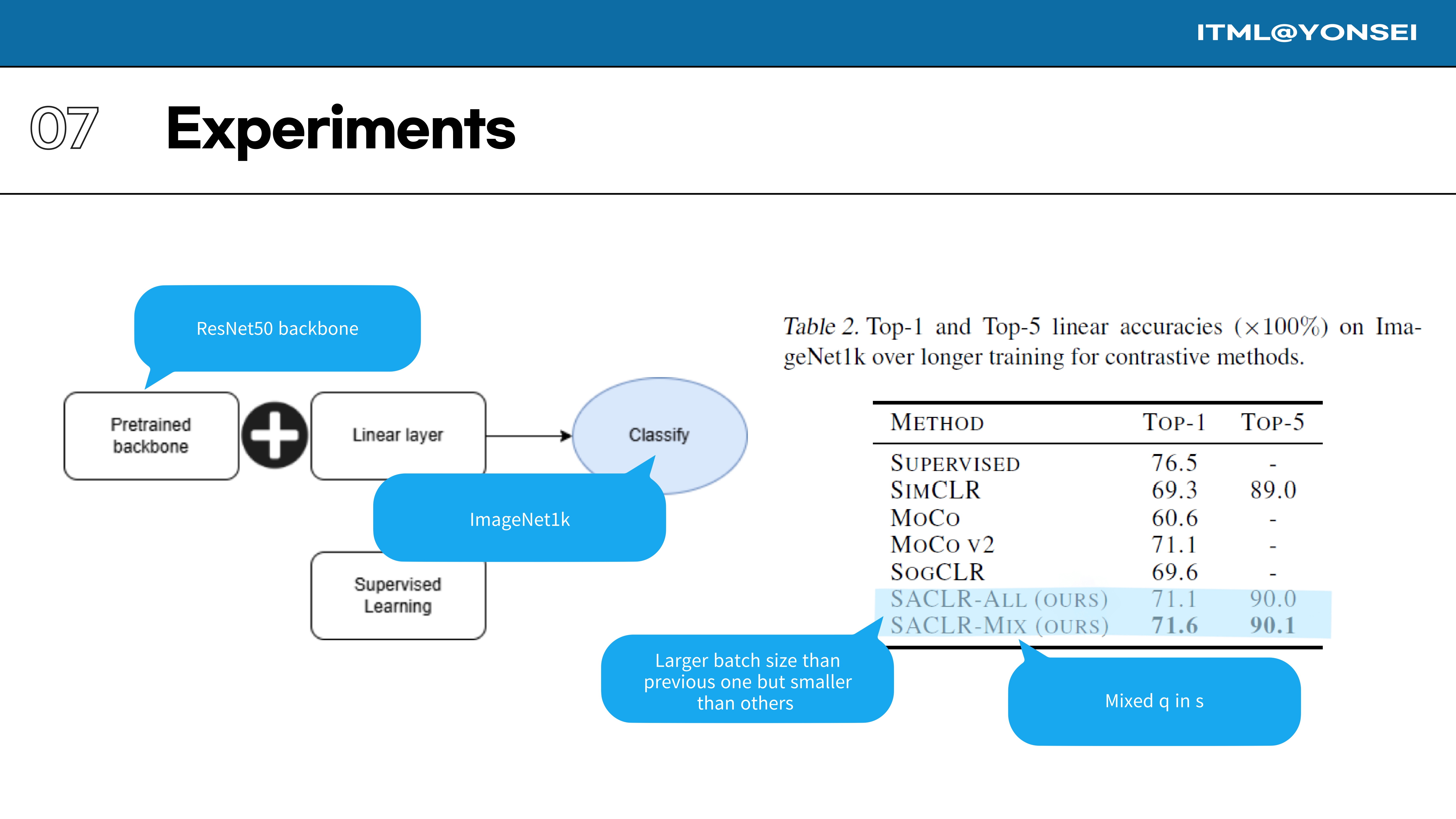
This table shows results for longer training, with SACLR-MIX surpassing SimCLR and SogCLR in this setup. However, reviewers found this comparison inadequate as well. Reviewer gz9D pointed out that results for top-performing methods like VICReg and Barlow Twins from other benchmark papers were significantly higher. The authors argued their goal was primarily efficiency without heavy tuning, but this did not overcome the concerns about the weak comparison set.

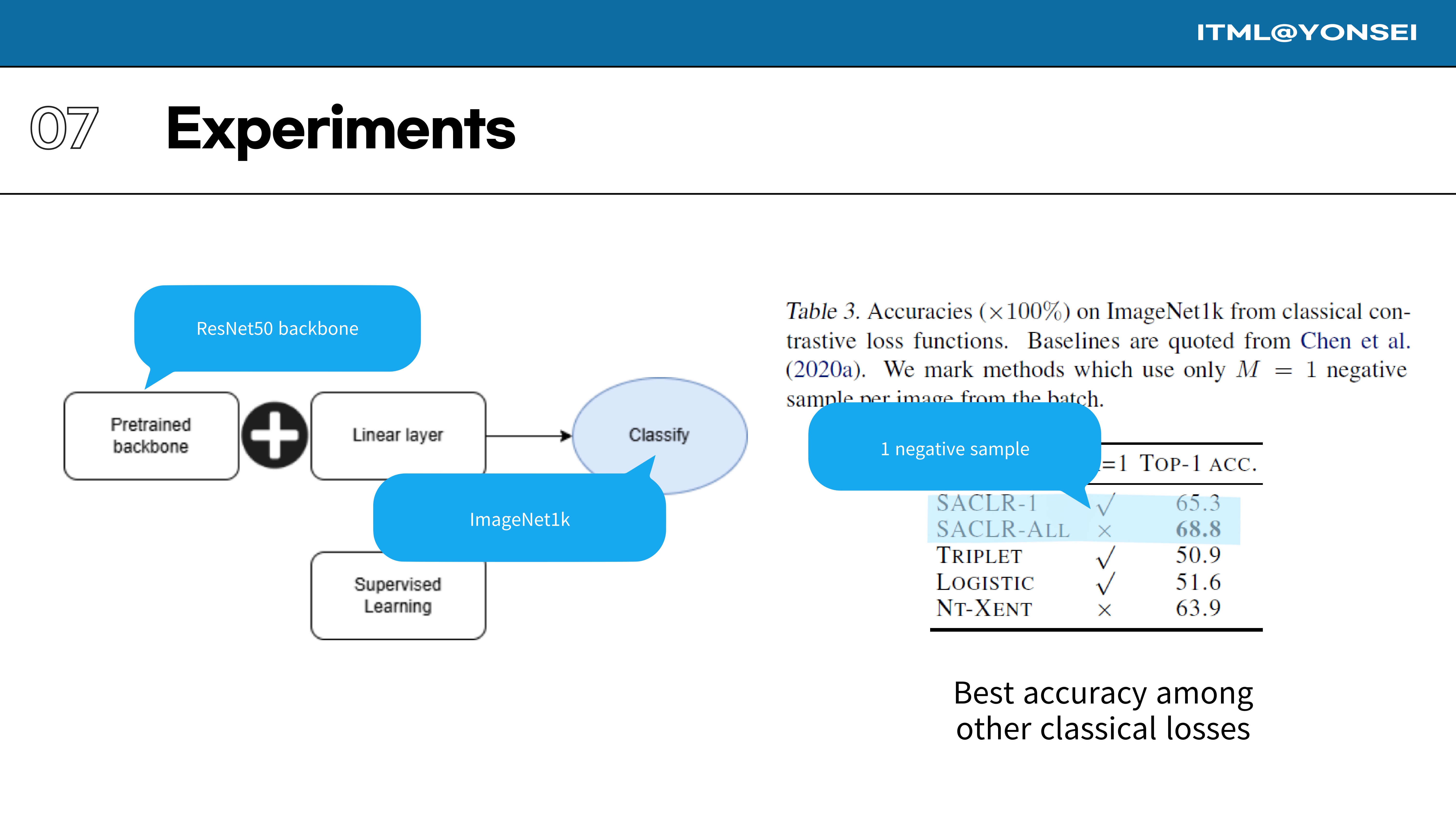
This experiment in Table 3 specifically investigates performance when using only a single negative sample (M=1) per image. SACLR-1 achieves a Top-1 accuracy of 65.3%, significantly outperforming classical contrastive losses like Triplet and Logistic loss under the same constraint.

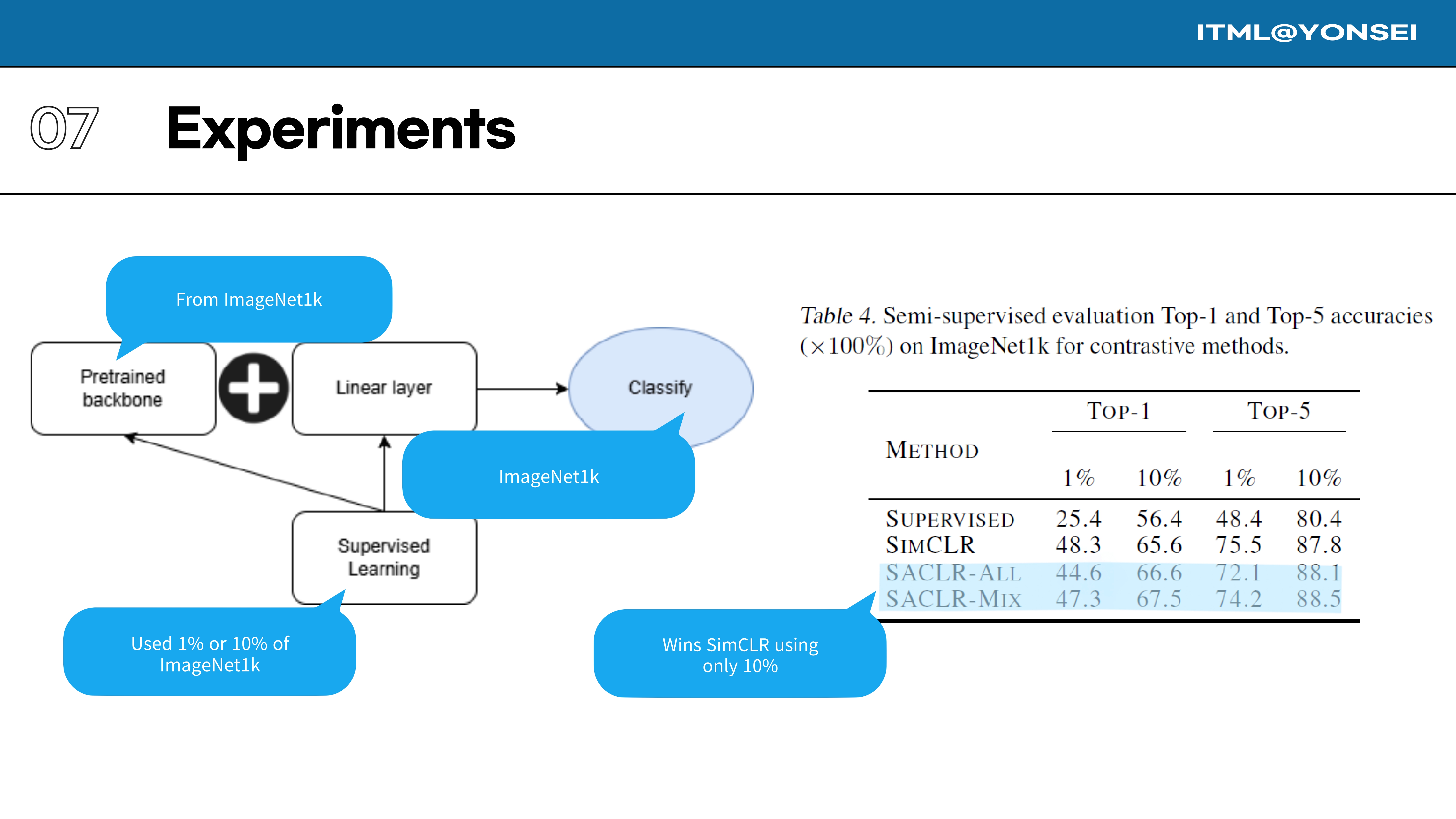
This table evaluates semi-supervised learning performance, showing SACLR’s strength in data-limited regimes. It is worth noting that the initial submission focused almost exclusively on linear evaluation. Reviewers Tx4K and gz9D strongly recommended including more comprehensive evaluations like semi-supervised fine-tuning to provide a more complete picture, and the additional kNN and fine-tuning results were added to the paper in response.

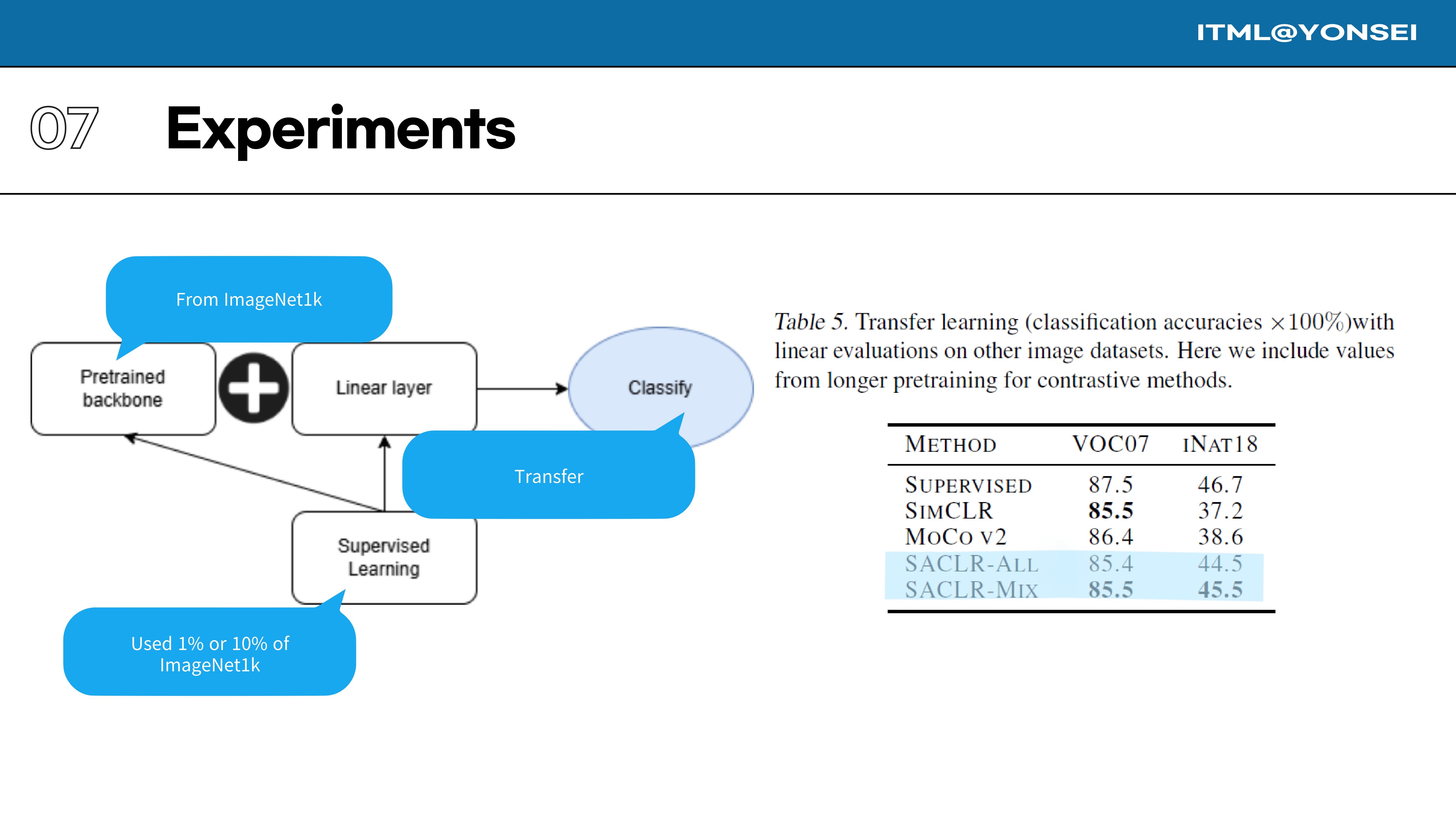
The learned representations are also evaluated on transfer learning classification tasks. As shown in Table 5, the representations learned by SACLR-ALL and SACLR-MIX transfer very well to other datasets like VOC07 and especially iNaturalist18, where they significantly outperform SimCLR and MoCo v2.

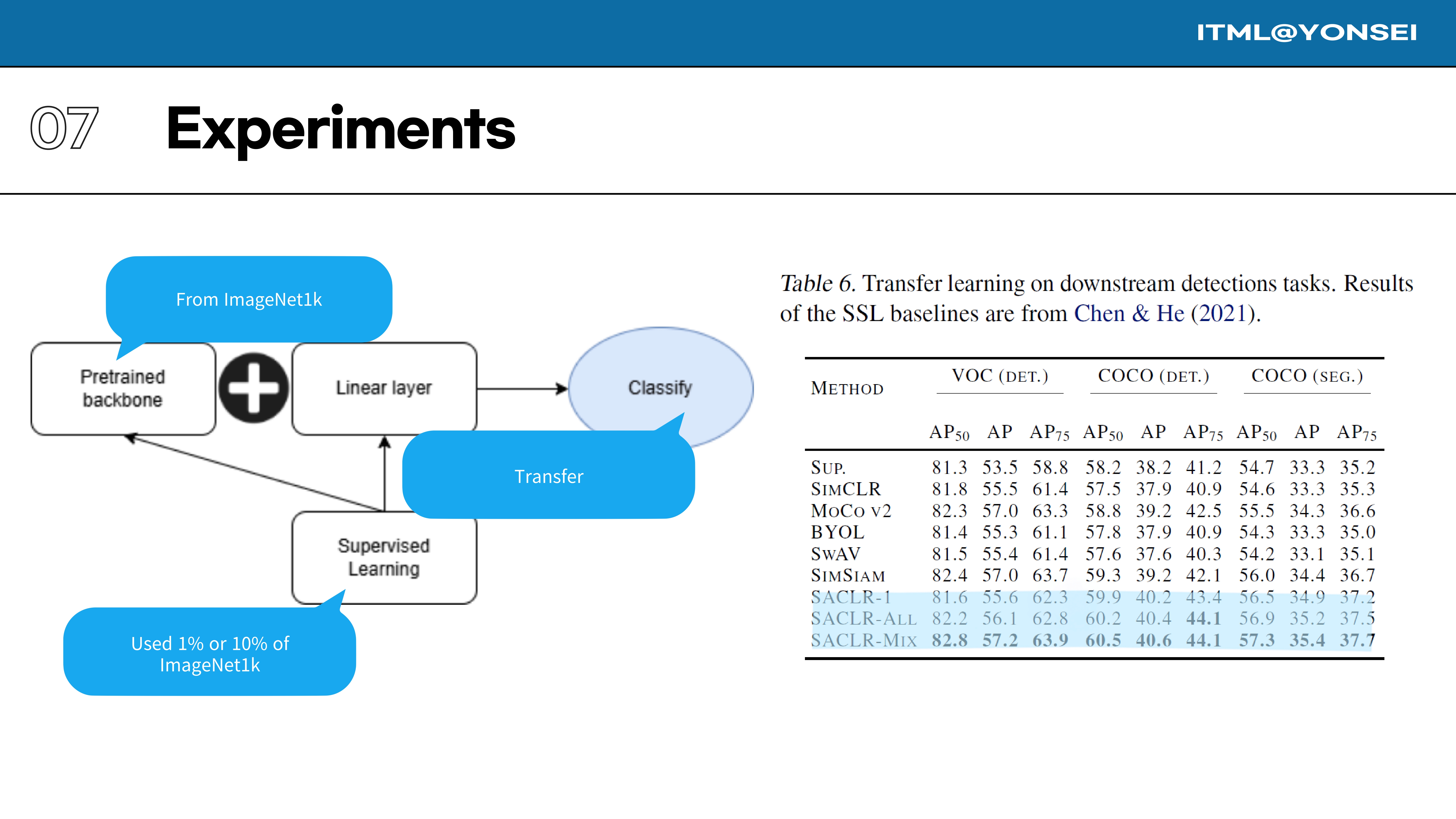
Table 6 shows transfer learning results on more complex downstream tasks: object detection and segmentation on VOC and COCO. Across all metrics, the SACLR variants are highly competitive and often outperform strong baselines like SimCLR, BYOL, and MoCo v2, with SACLR-MIX showing the strongest results overall.

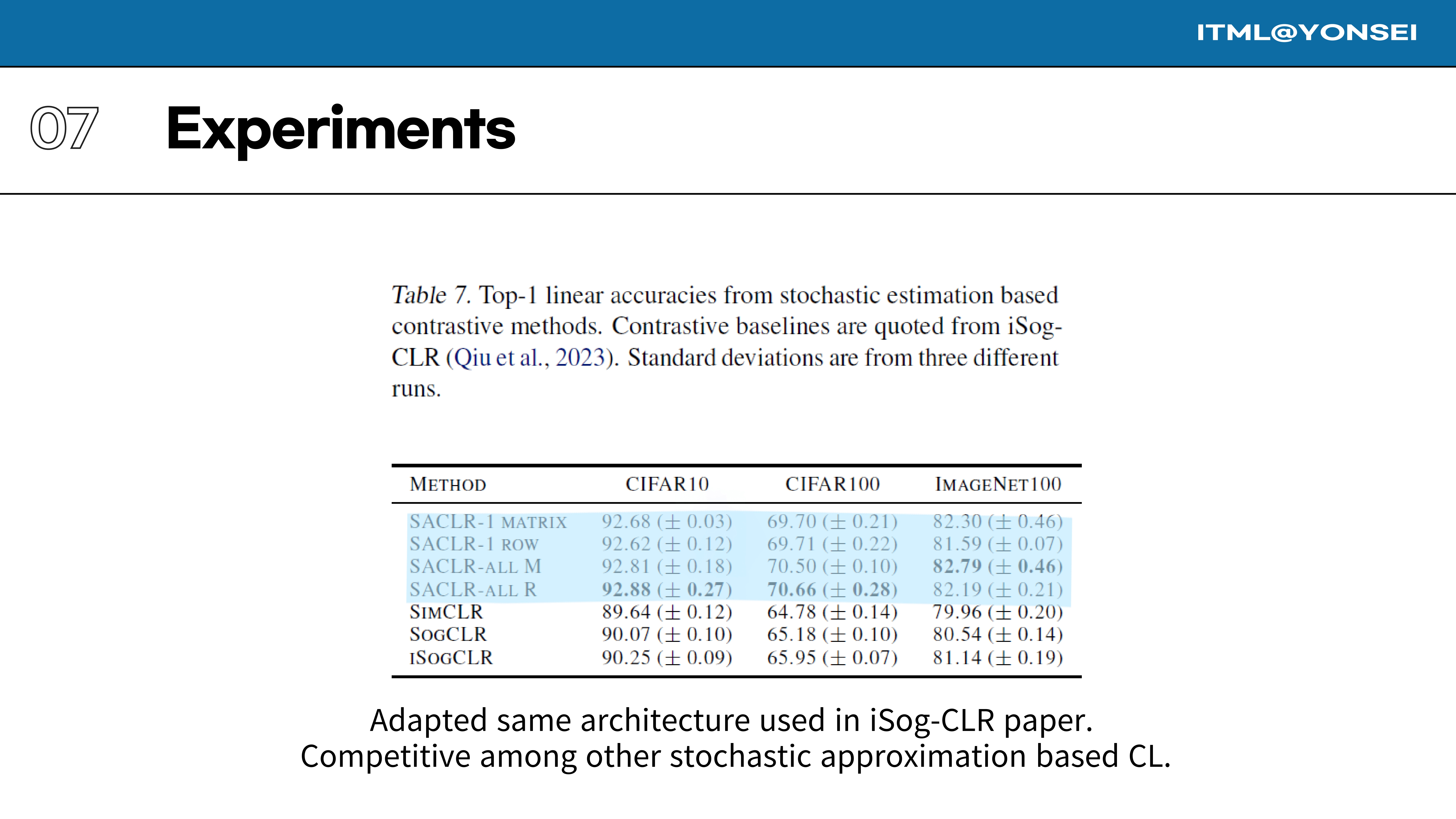
This table provides a direct comparison with other stochastic estimation-based contrastive methods, using an architecture similar to the iSog-CLR paper for a fair comparison. The results on CIFAR10, CIFAR100, and ImageNet100 show that both the matrix and row versions of SACLR are highly competitive, often achieving the best or second-best performance in this specific class of methods.

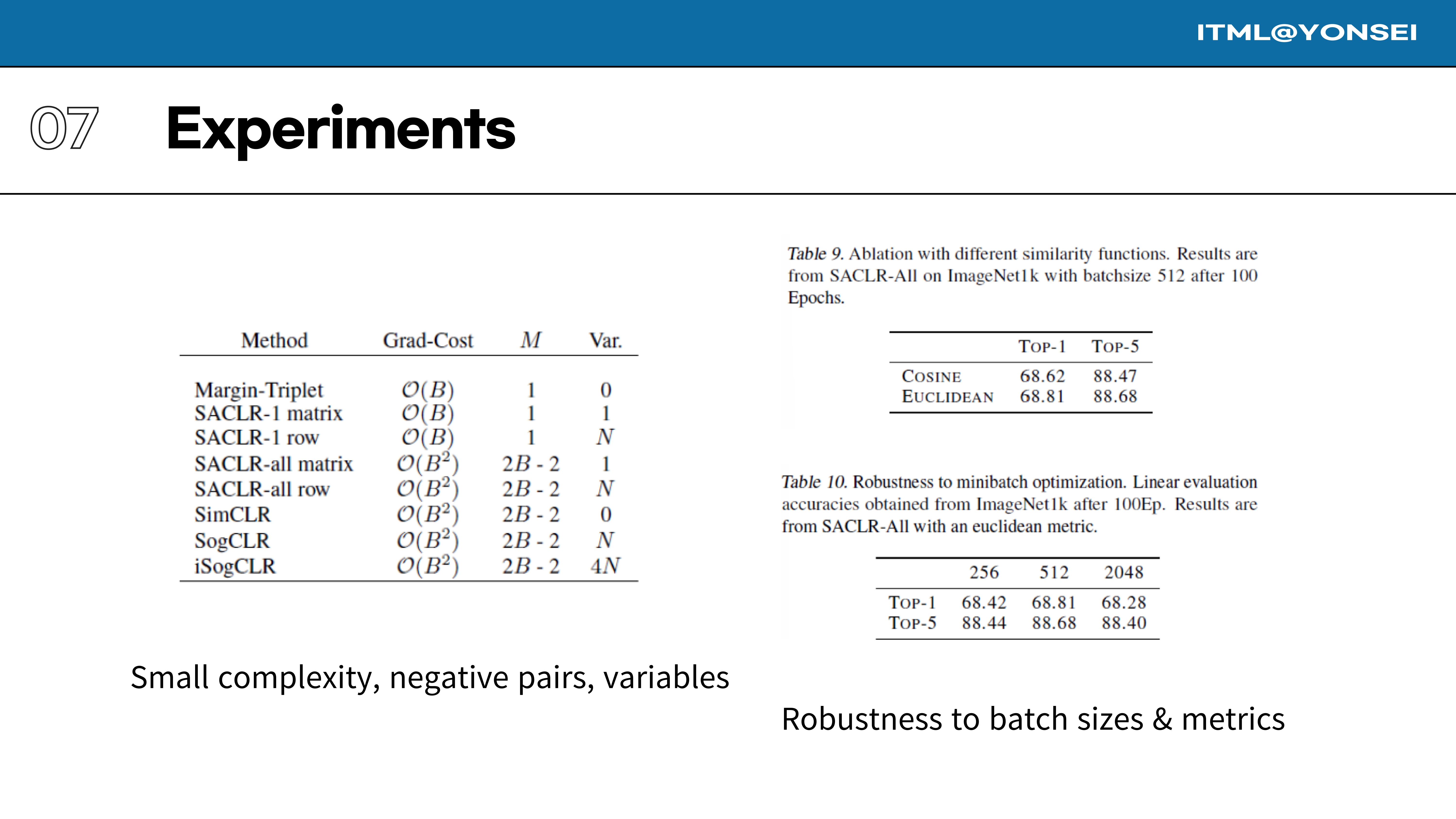
This slide presents several ablation studies on computational complexity and robustness. These experiments were largely added in response to direct reviewer feedback. Reviewers requested empirical data on runtime and memory to substantiate the paper’s efficiency claims, as well as a study on the impact of batch size to support the claim that SACLR performs well in small-batch settings. These tables represent the authors’ attempt to provide that missing evidence.