Max-Margin Token Selection in Attention Mechanism

Hello everyone, I’m Jungmook Kang at Yonsei University. Today, I’m excited to share a review of a fascinating paper that was recently accepted to NeurIPS, which delves into the theoretical underpinnings of the attention mechanism. Let’s get started.

The title of the paper is “Max-Margin Token Selection in Attention Mechanism.” This work comes from our lab here at Yonsei University, and it explores the question of why attention works the way it does.

So, let’s begin with the motivation for this research. What prompted us to look into this?

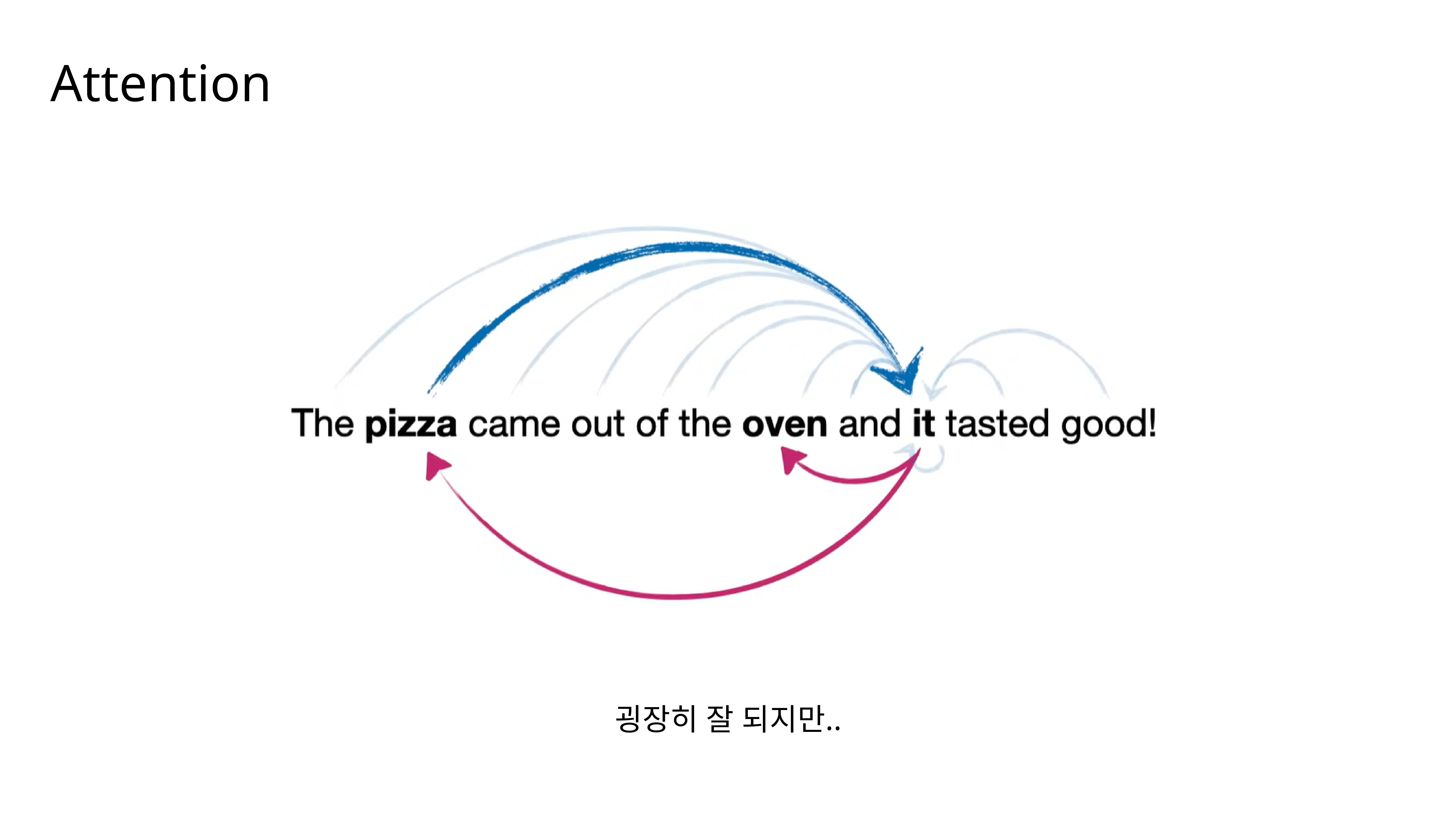
We all know that the attention mechanism is incredibly effective. For a sentence like “The pizza came out of the oven and it tasted good!”, attention can correctly associate “it” with “pizza.” It works remarkably well… but the story doesn’t end there.

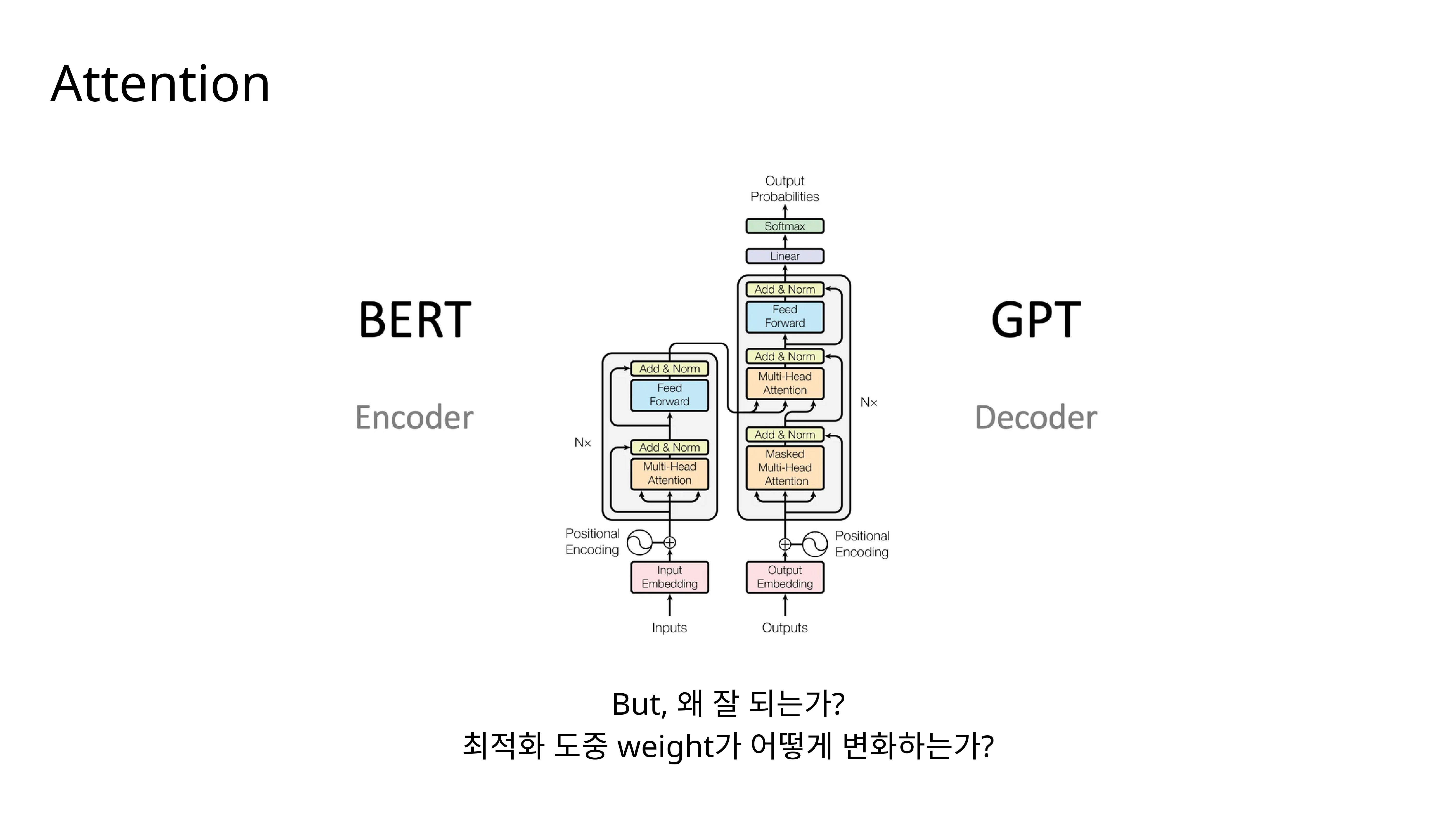
When we look at the standard Transformer architecture, which powers models like BERT and GPT, we see a complex system of encoders and decoders with multiple layers of multi-head attention. This raises some fundamental questions: Why is this architecture so successful? And more specifically, what is happening to the model’s weights during the optimization process that leads to this success?

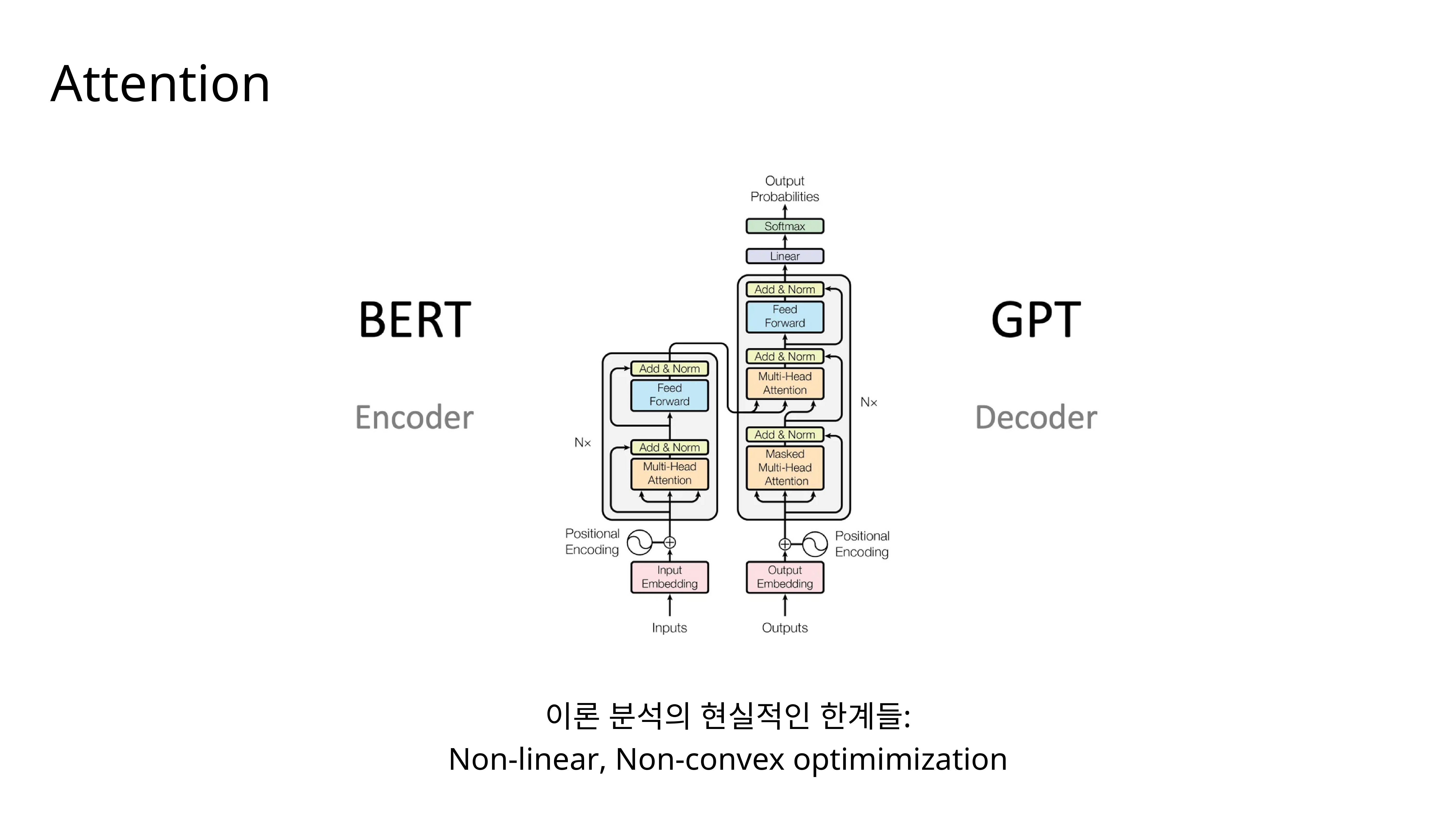
Analyzing this architecture theoretically is very challenging. The optimization problem is both non-linear, due to functions like Softmax, and non-convex. This makes it extremely difficult to describe the training dynamics with traditional methods.

To tackle this, we turn to the concept of “Implicit Bias.” This is a phenomenon where the optimization algorithm itself—like Gradient Descent—has a preference for a certain type of solution, even when there’s no explicit regularization term in the loss function telling it to do so.

This leads us to the central question of our research: What is the implicit bias of the attention model? What kind of solution does it naturally favor?

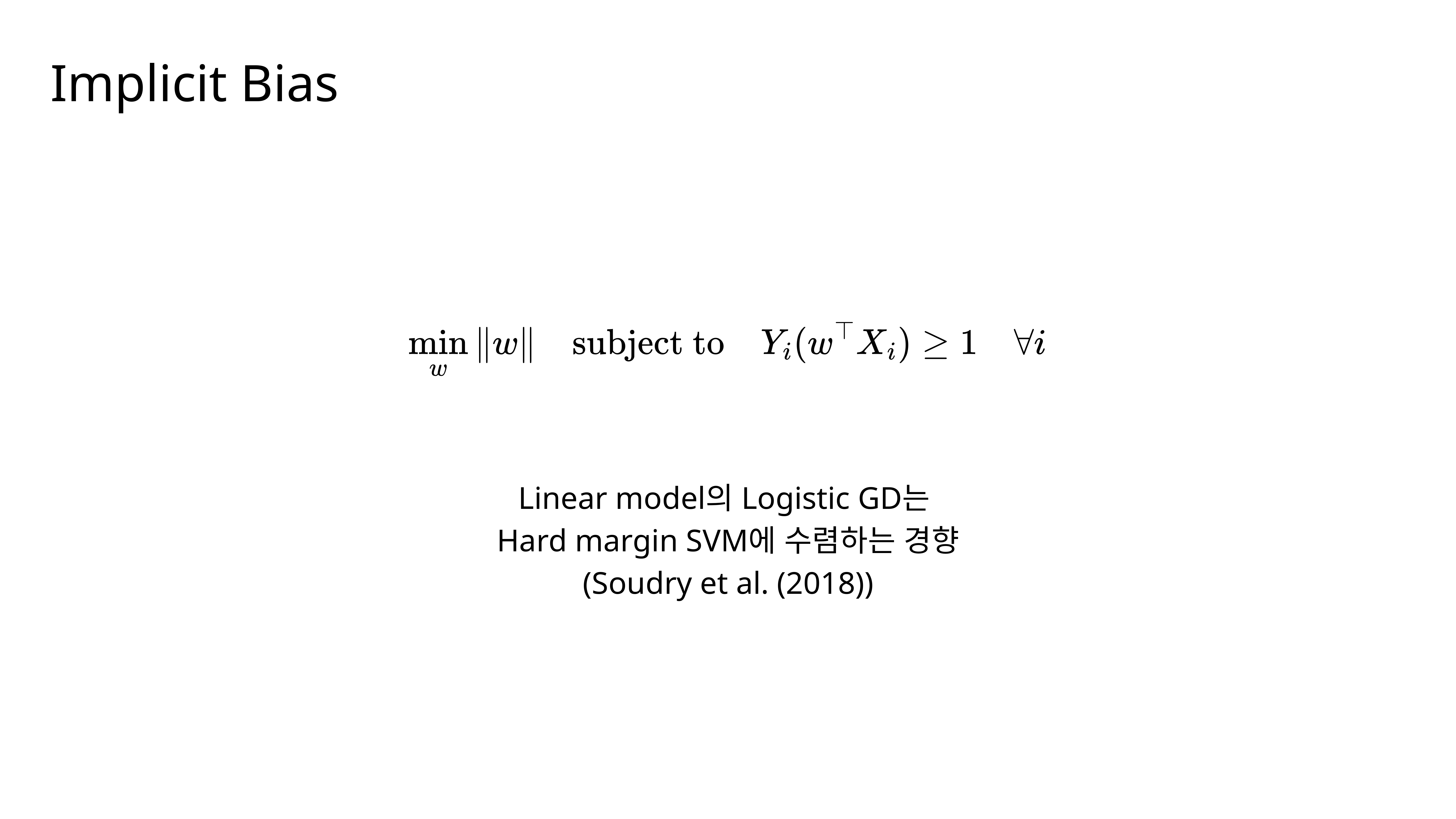
We can get a clue from simpler models. It’s a known result from Soudry et al. (2018) that when you train a linear model with logistic loss using gradient descent, the solution tends to converge towards the one you’d get from a hard-margin Support Vector Machine (SVM). The goal of a hard-margin SVM is to find the hyperplane that maximizes the distance, or margin, to the nearest data points.

So, we formed a hypothesis: Could it be that the implicit bias of the much more complex attention model is also related to a hard-margin SVM solution?

Here’s a core idea. We observe that attention has a tendency to focus on a small number of important tokens. We believe the principle guiding this selection is related to maximizing a margin. For instance, to distinguish between a cat and a dog, you might focus on the shape of the ’ears’ because that feature provides the clearest separation, the largest ‘margin,’ between the two classes.

This brings us to the first main part of the analysis, where we explore the idea of global and local margin maximization within the attention mechanism.

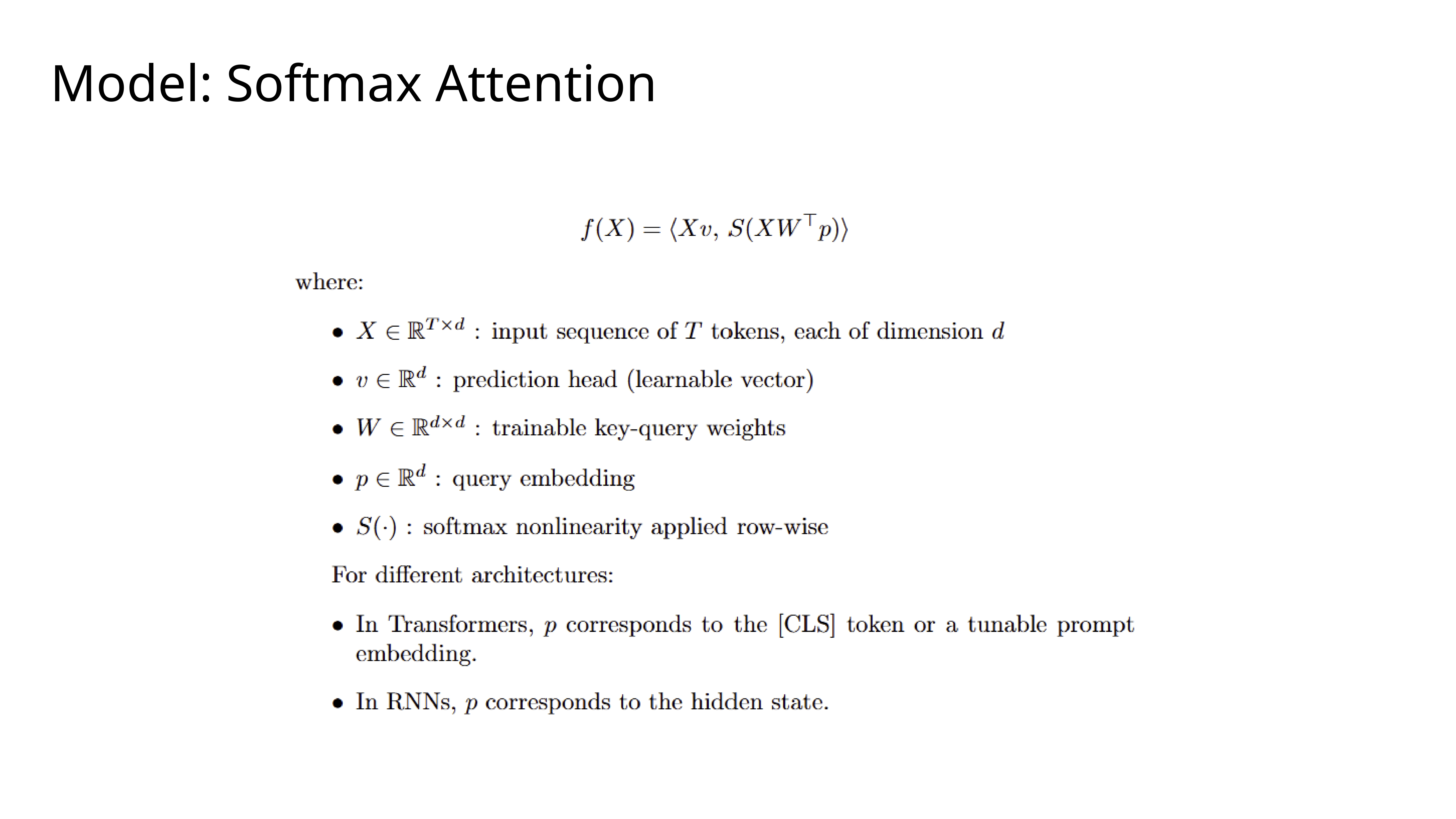
To make the analysis tractable, we start with a simplified Softmax Attention model. The function f(X) takes an input sequence X and computes a final output. The key learnable parameters are p, the query embedding, and W, the key-query weights. In Transformers, p can be thought of as the embedding for the [CLS] token.

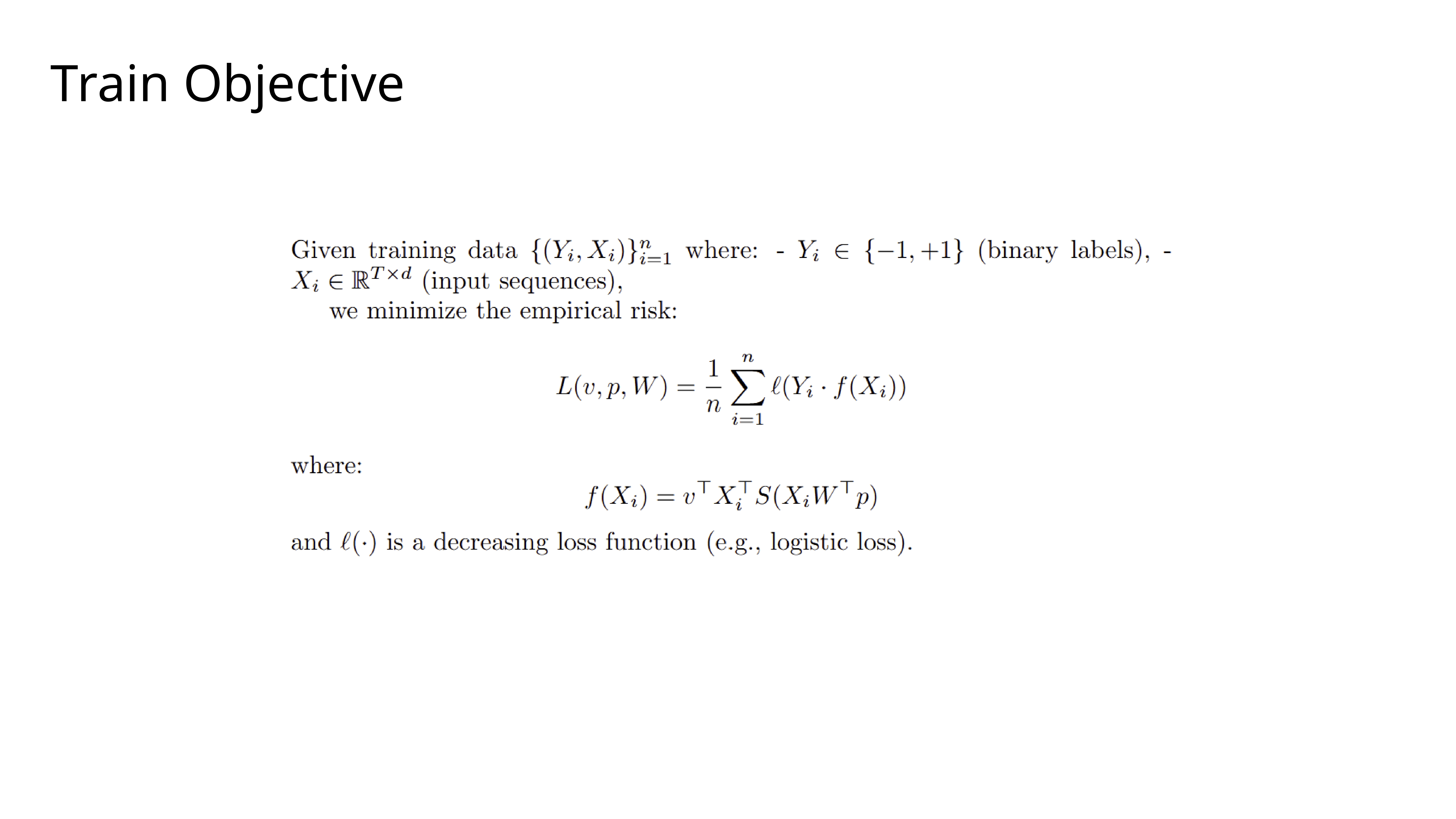
Our training objective is to minimize the empirical risk for a binary classification task. We use a standard setup with input sequences X and labels Y, and a decreasing loss function like logistic loss. The model’s prediction f(Xi) is a function of the learnable parameters v, p, and W.

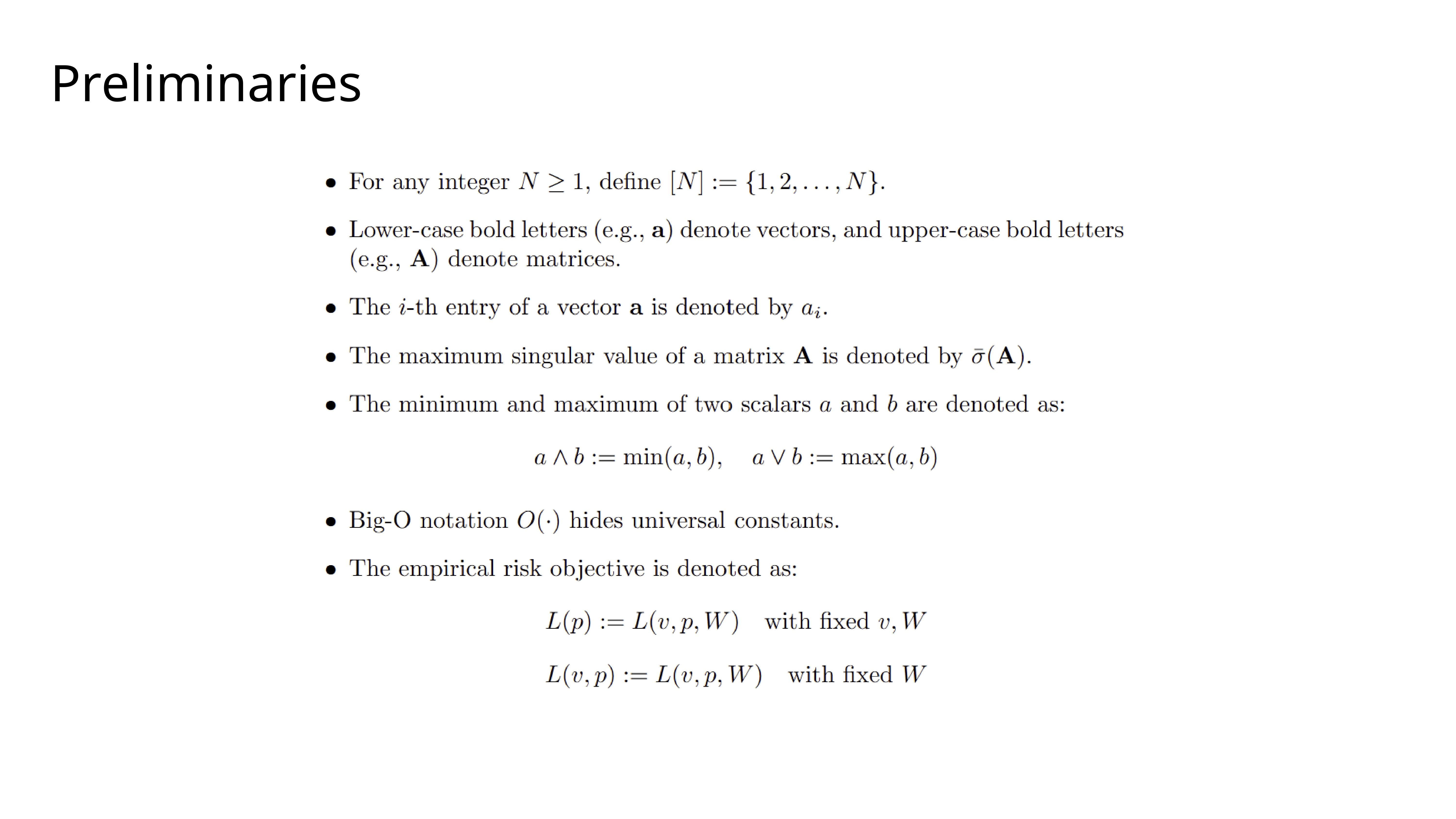
Here, I’ll just quickly go over some of the mathematical notation we use throughout the paper. We use standard conventions for vectors and matrices, and we’ll use simplified notations like L(p) to denote the risk when v and W are fixed.

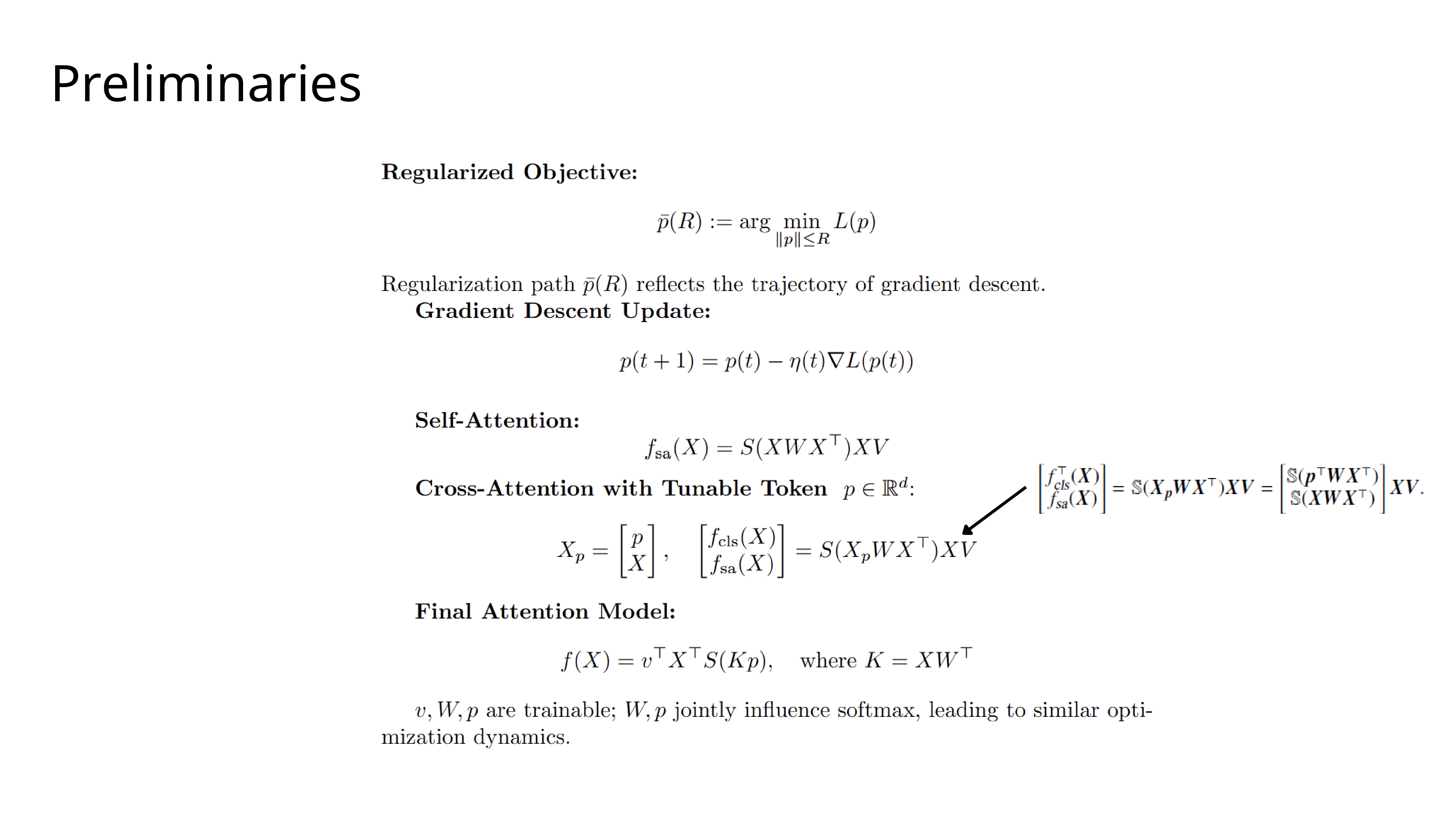
Our approach involves studying the regularization path, which is the path of the solution p as we increase its allowed norm, R. This path mirrors the trajectory of gradient descent. We analyze a final attention model where the trainable parameters W and p jointly influence the softmax, leading to similar optimization dynamics.

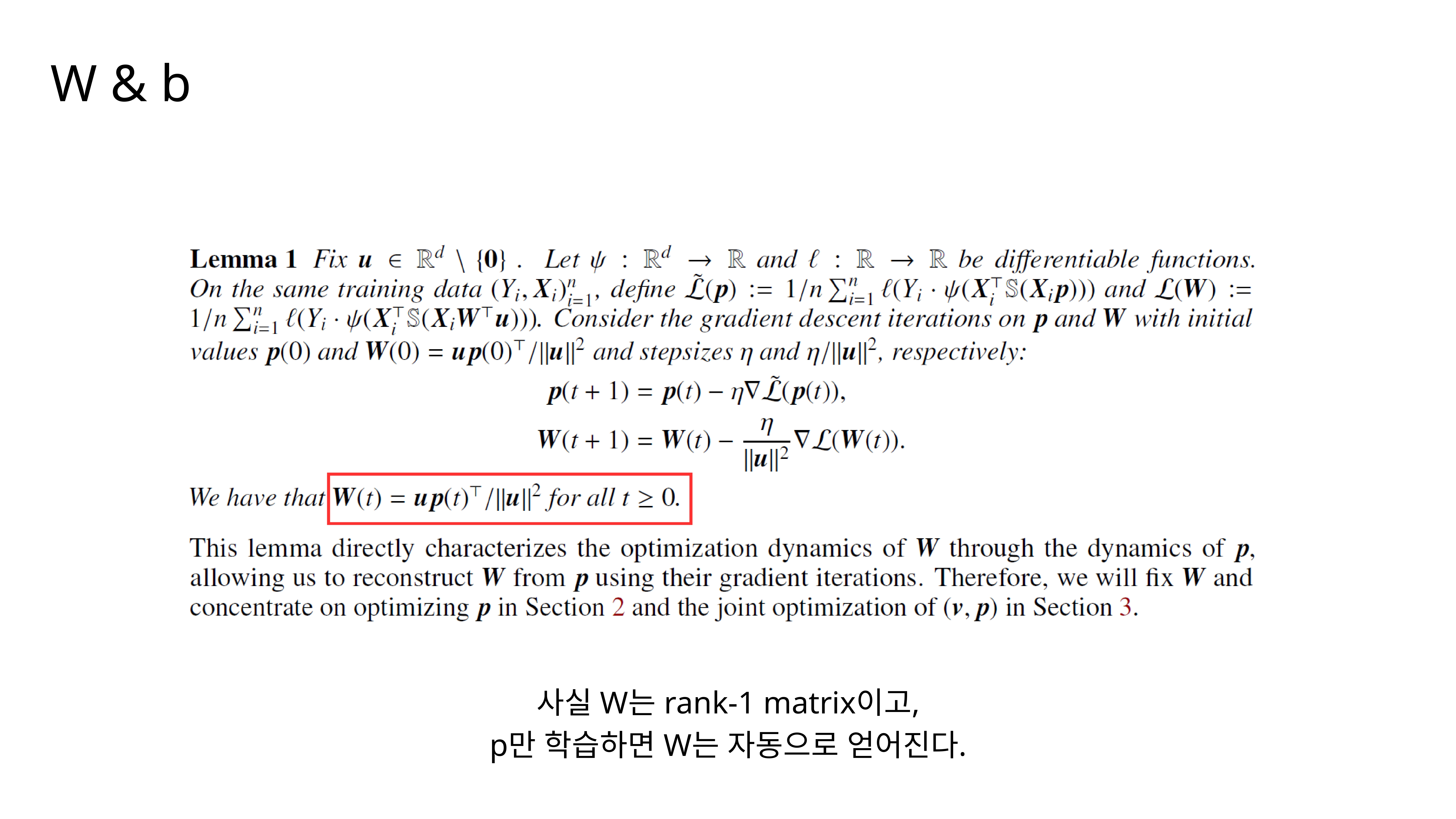
This brings us to Lemma 1, which is a crucial simplification. It states that the weight matrix W is effectively a rank-1 matrix and its learning dynamics are completely determined by the vector p. This is very important because it means we can fix W and focus our entire analysis on the optimization of p.

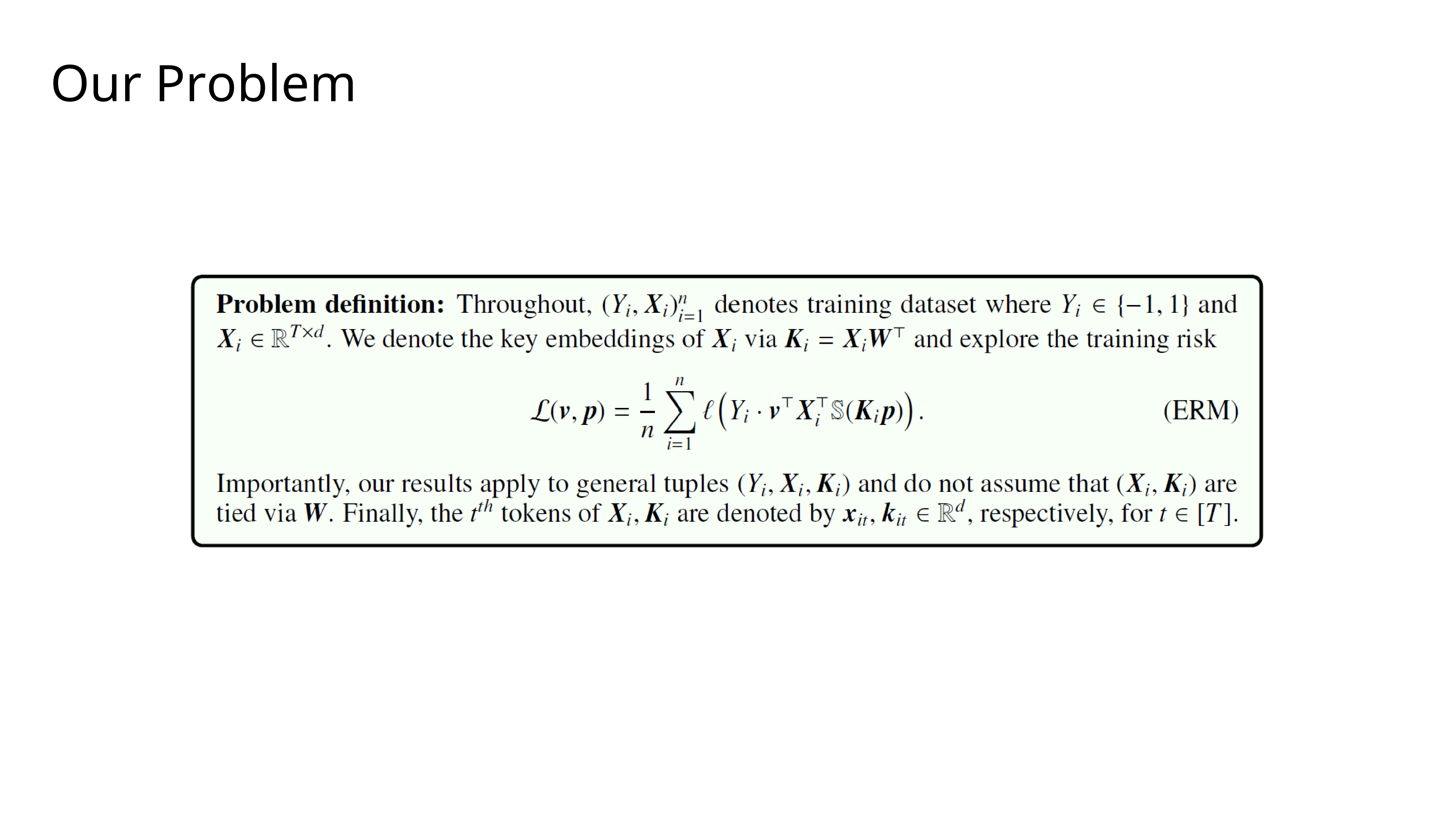
So, we can formally define our problem. We are exploring the training risk L(v, p) where the key embeddings Ki are derived from the input Xi. For the analysis, we can even treat Xi and Ki as separate entities.

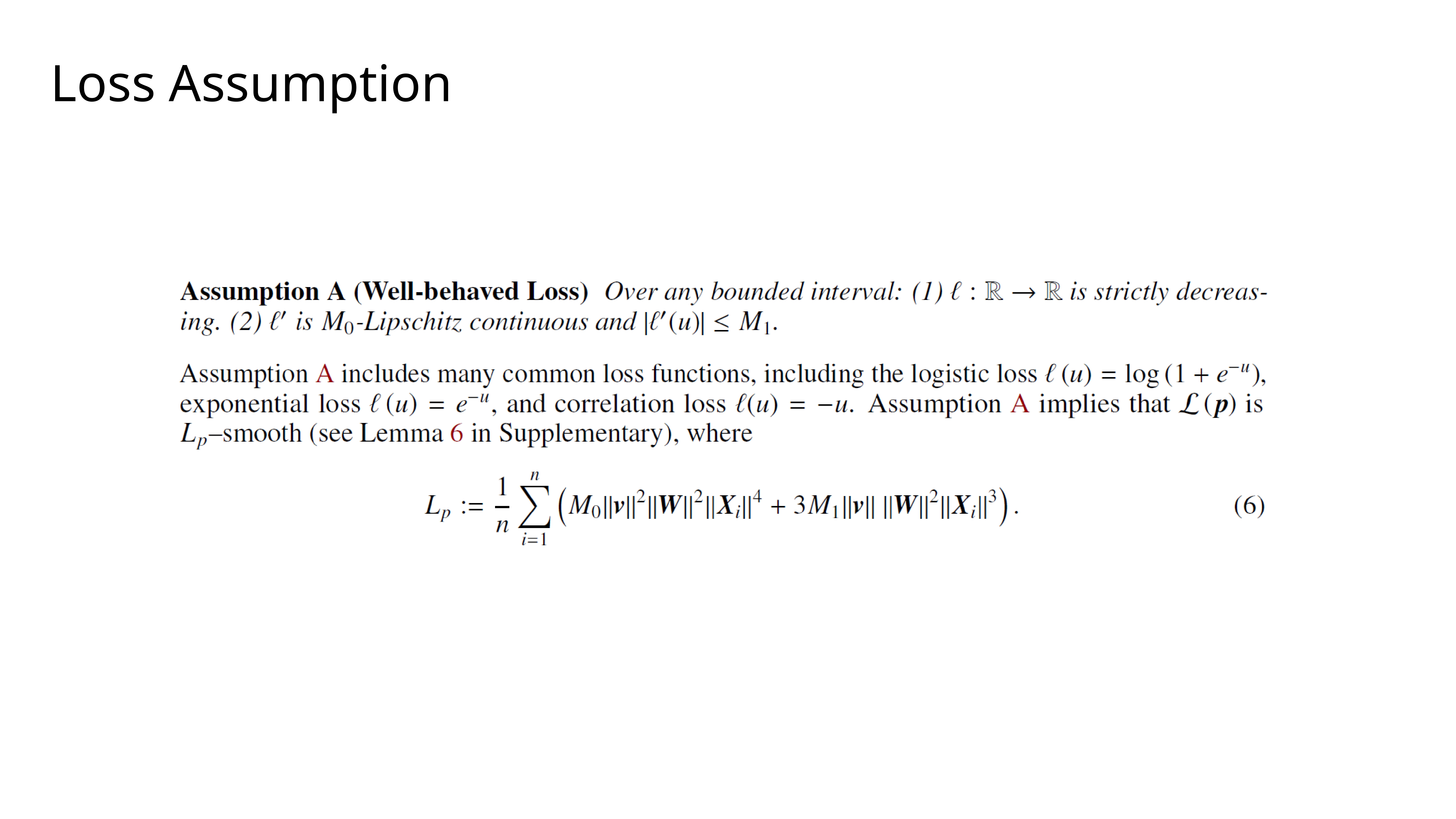
To ensure our proofs hold, we need Assumption A. This is a standard assumption that requires our loss function l to be well-behaved—specifically, it must be strictly decreasing and have a Lipschitz-continuous derivative. Common functions like logistic loss and exponential loss satisfy this condition.

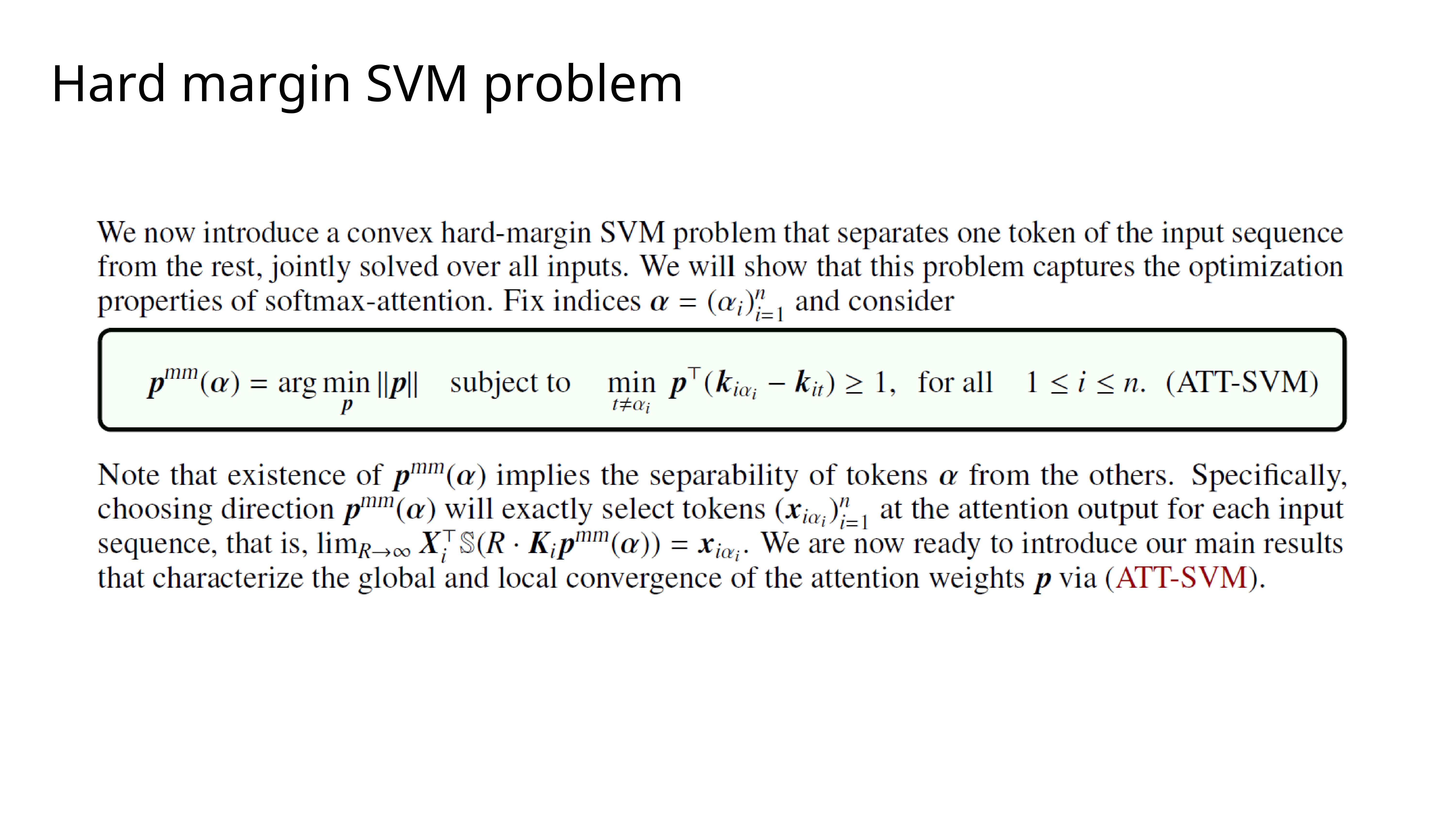
Now, we introduce the central piece of our theory: a hard-margin SVM problem, which we call ATT-SVM. The goal here is to find a direction p that, for each input sequence, separates one chosen token (k_iαi) from all other tokens (k_it) by a margin of at least 1. We will show that the optimization of softmax attention is effectively trying to solve this problem.

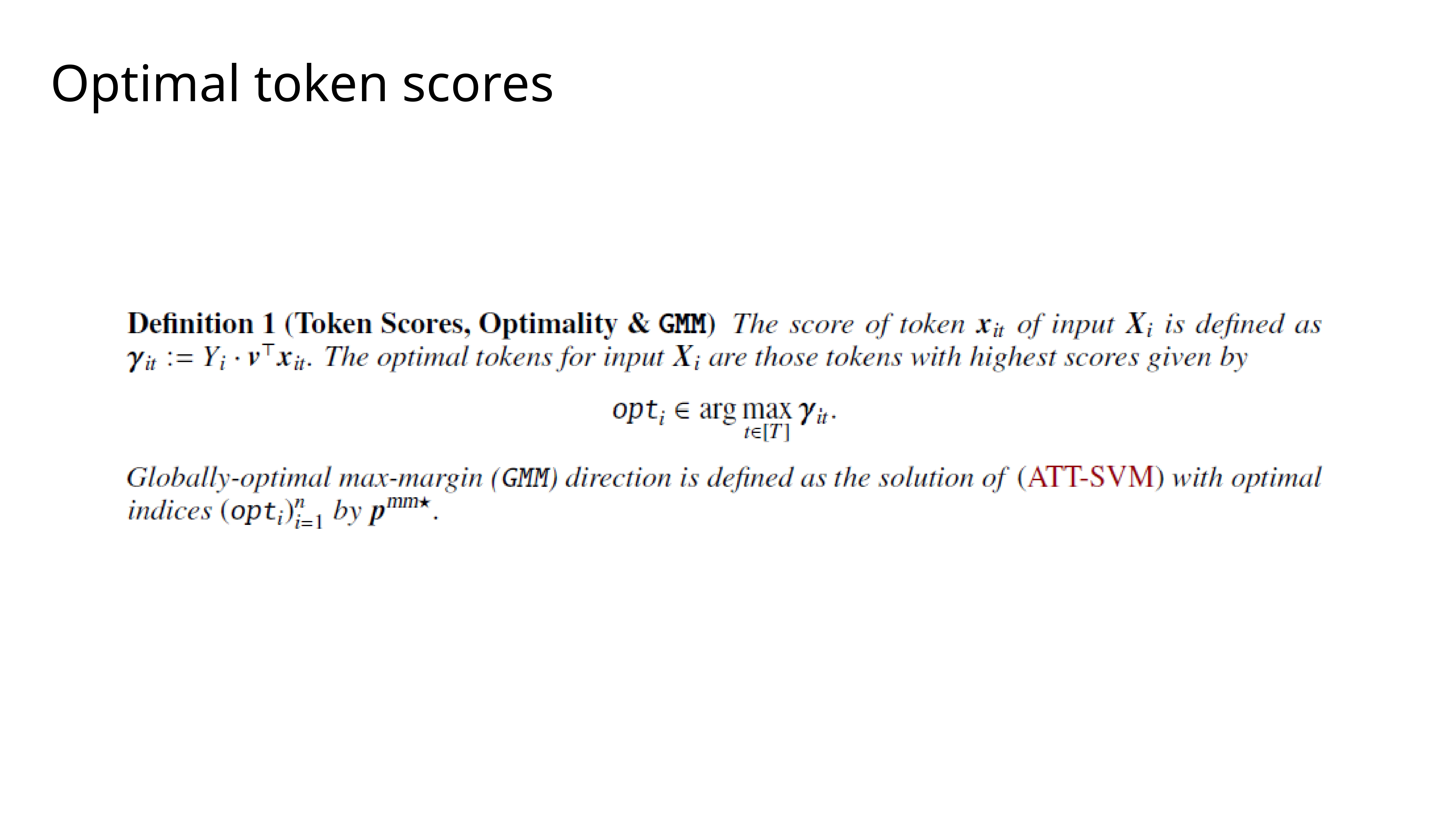
To formalize this, we define the score of a token (γ_it) as its contribution to the final correct prediction. The optimal tokens are naturally the ones with the highest scores for each input. The Globally-Optimal Max-Margin (GMM) direction, denoted p^mm*, is then the solution to our ATT-SVM problem when we choose these optimal tokens.

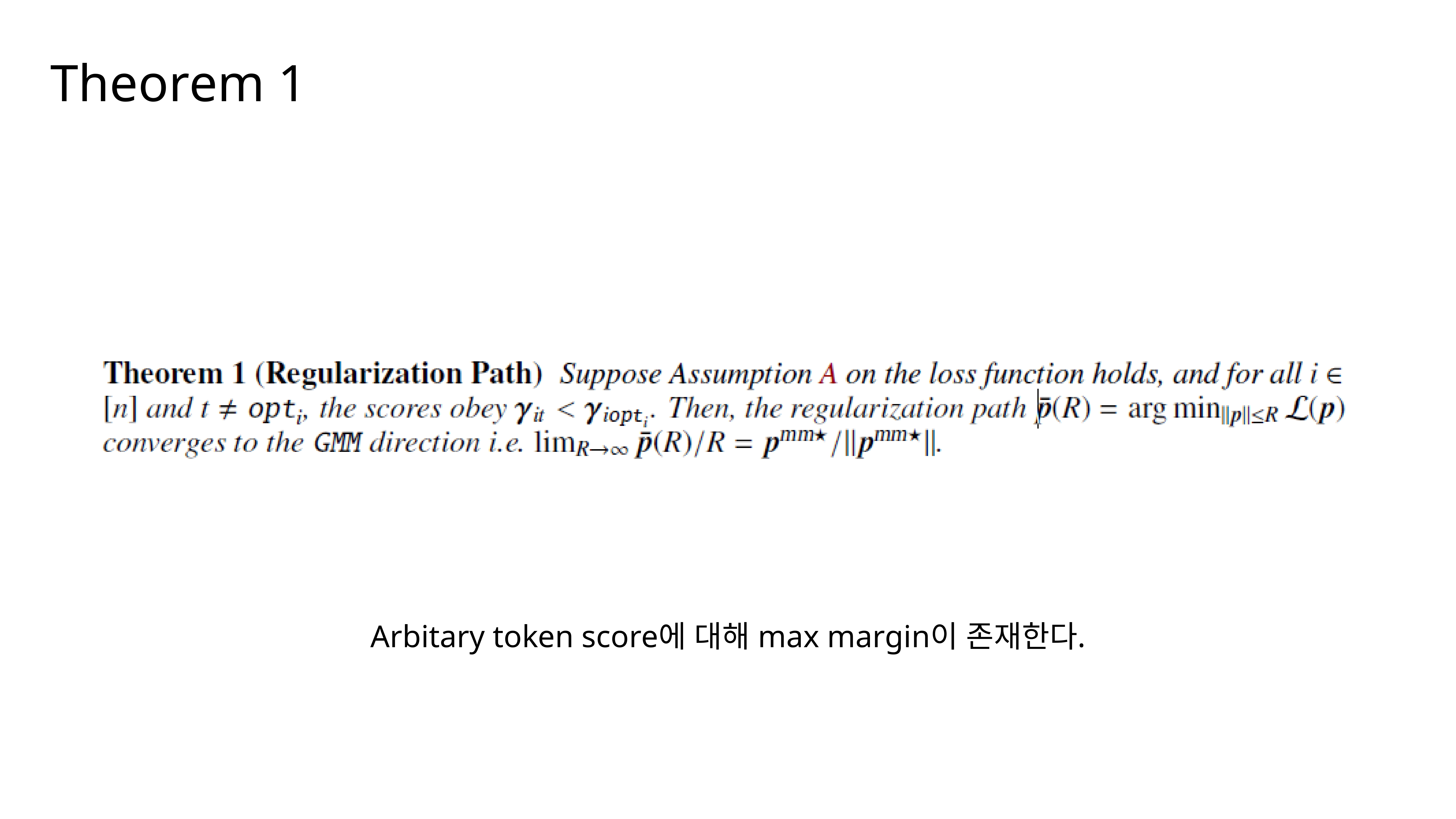
Theorem 1 is our first main result. It states that the regularization path—the sequence of solutions as we increase the norm R—converges in direction to this GMM solution, p^mm*. In simple terms, as the optimization progresses and the norm of p grows, its direction aligns with the direction that best separates the highest-scoring tokens from the rest.

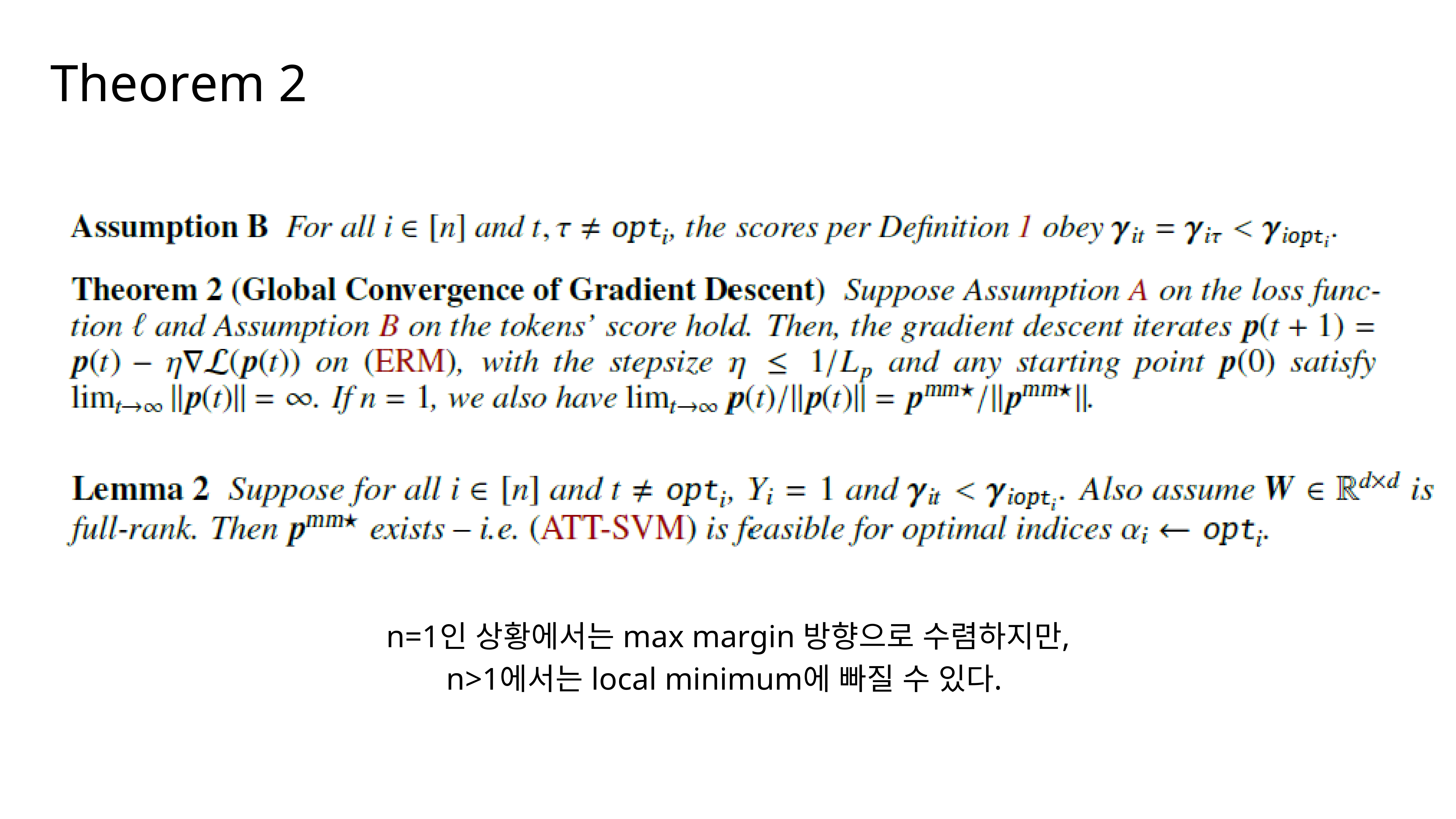
Theorem 2 looks at the convergence of gradient descent directly. It says that under our assumptions, the norm of the weight vector p will grow towards infinity during training. Critically, for the simple case of a single training example (n=1), the direction of p converges to the GMM direction. However, for n > 1, it’s possible for the optimization to get trapped in a local minimum.

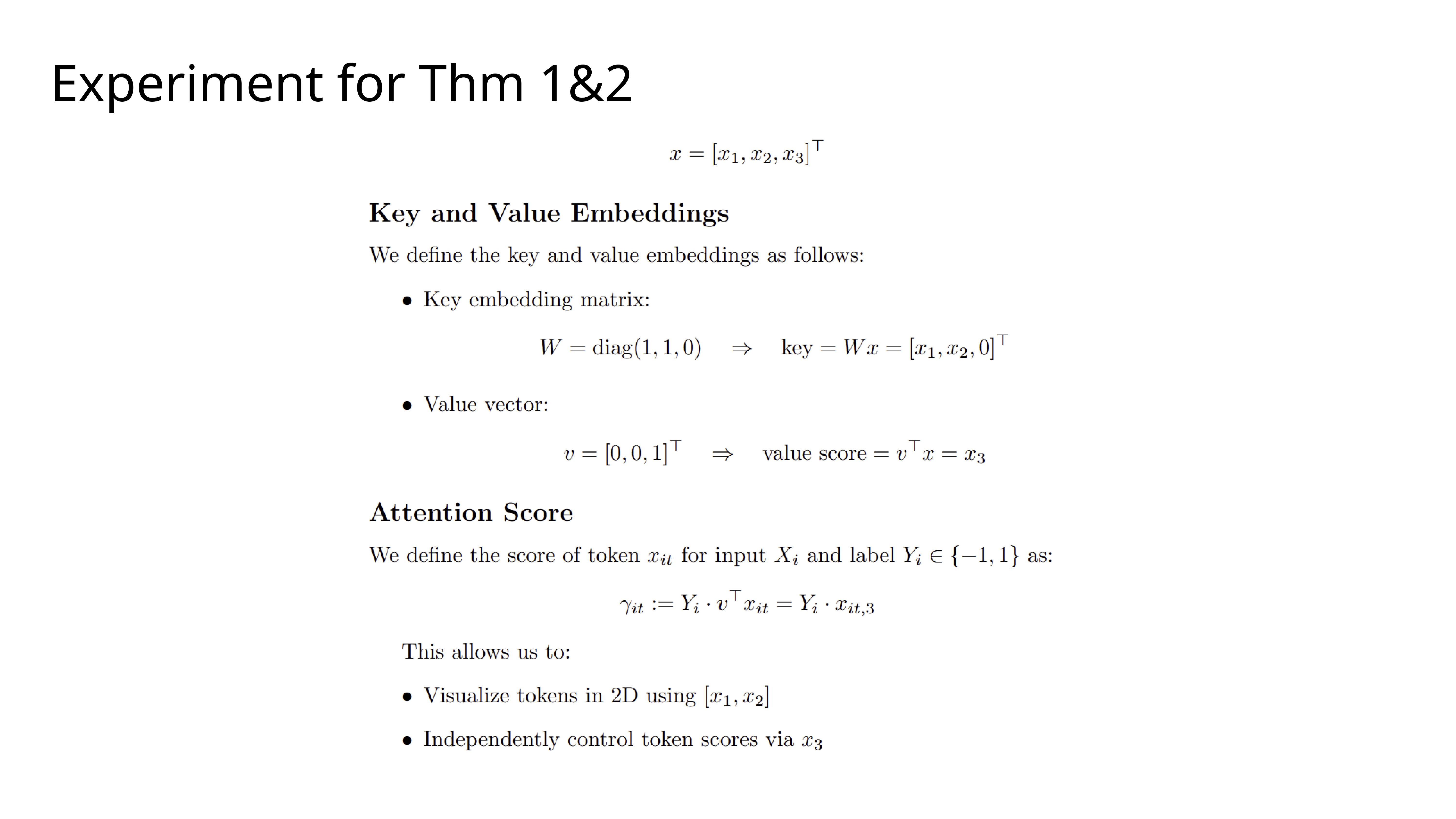
To test these theorems, we designed a simple experiment. We created synthetic data with three tokens, where we can visualize their key embeddings in 2D and independently control their scores using a third dimension. This lets us clearly see what’s happening.

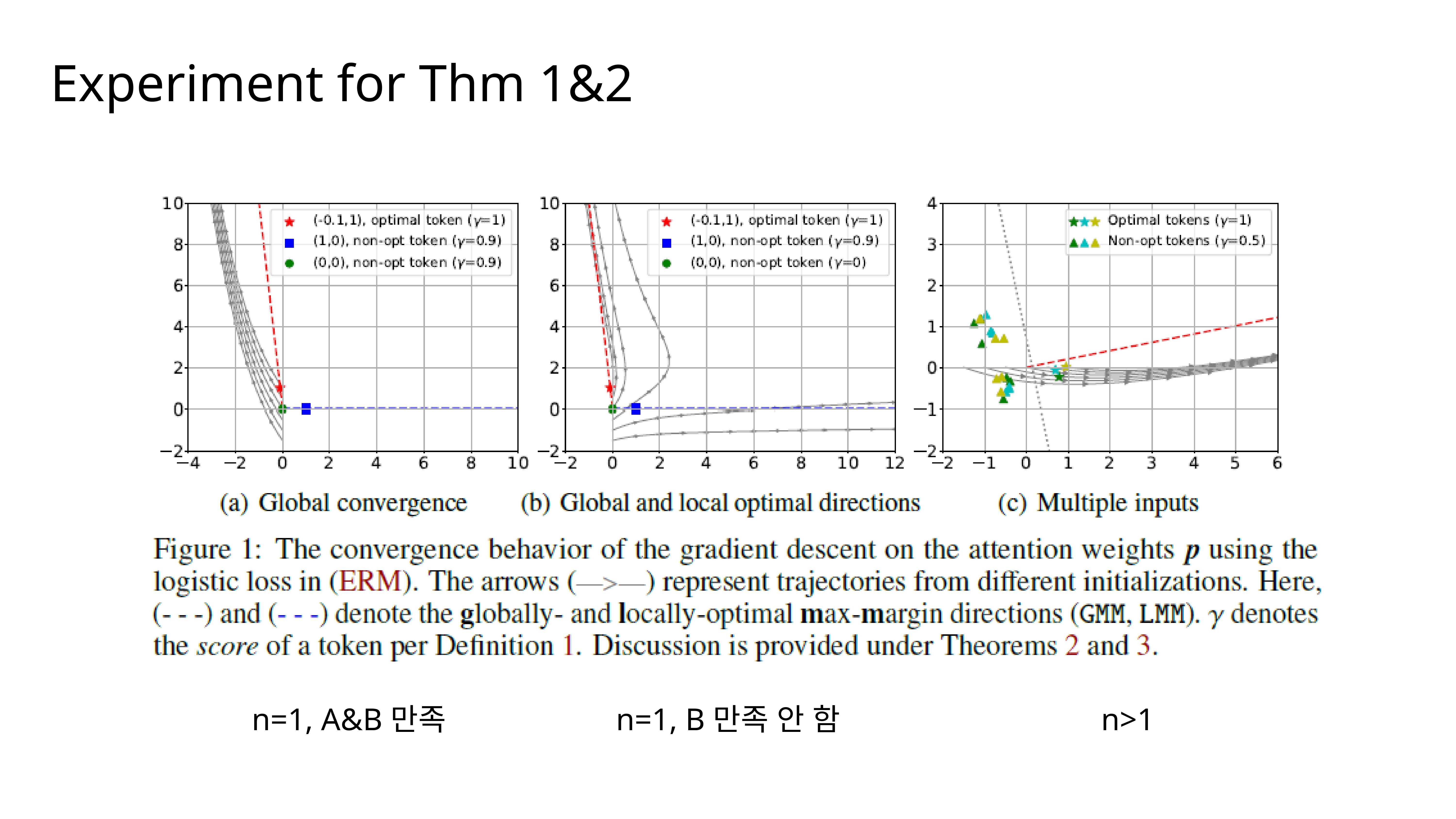
These plots show the results. In Figure (a), where the conditions for global convergence are met, we see that all gradient descent trajectories (the grey arrows) correctly converge to the GMM direction (the red dashed line). In (b), we’ve changed the scores so that a locally optimal solution exists, and we see some trajectories get stuck there instead. Figure (c) shows the more complex scenario with multiple inputs, where finding the joint GMM solution is harder.

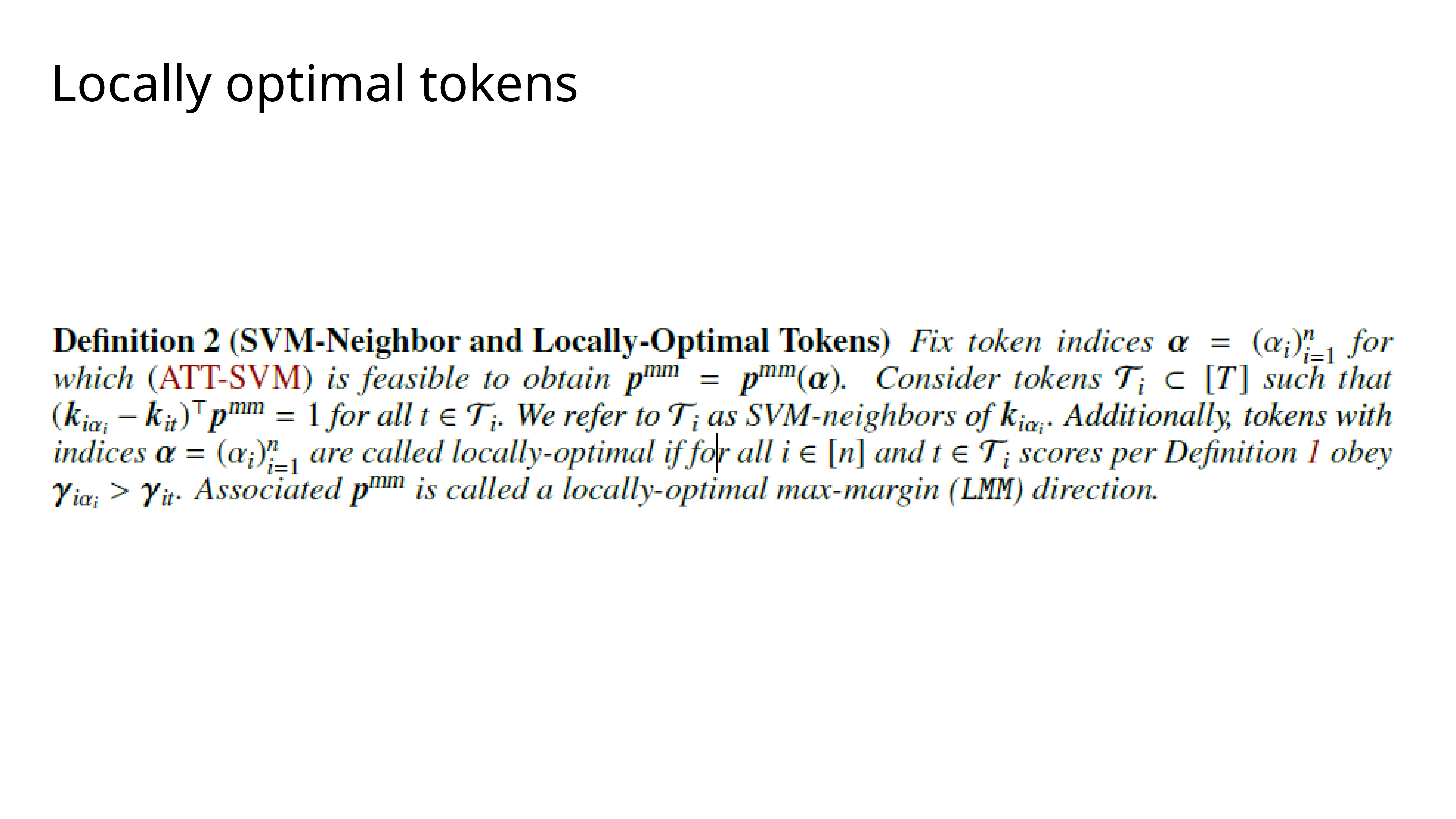
This brings us to the idea of locally-optimal tokens. These are tokens that might not be the highest-scoring ones globally, but they form a stable solution for the ATT-SVM problem. The direction associated with them is a locally-optimal max-margin (LMM) direction.

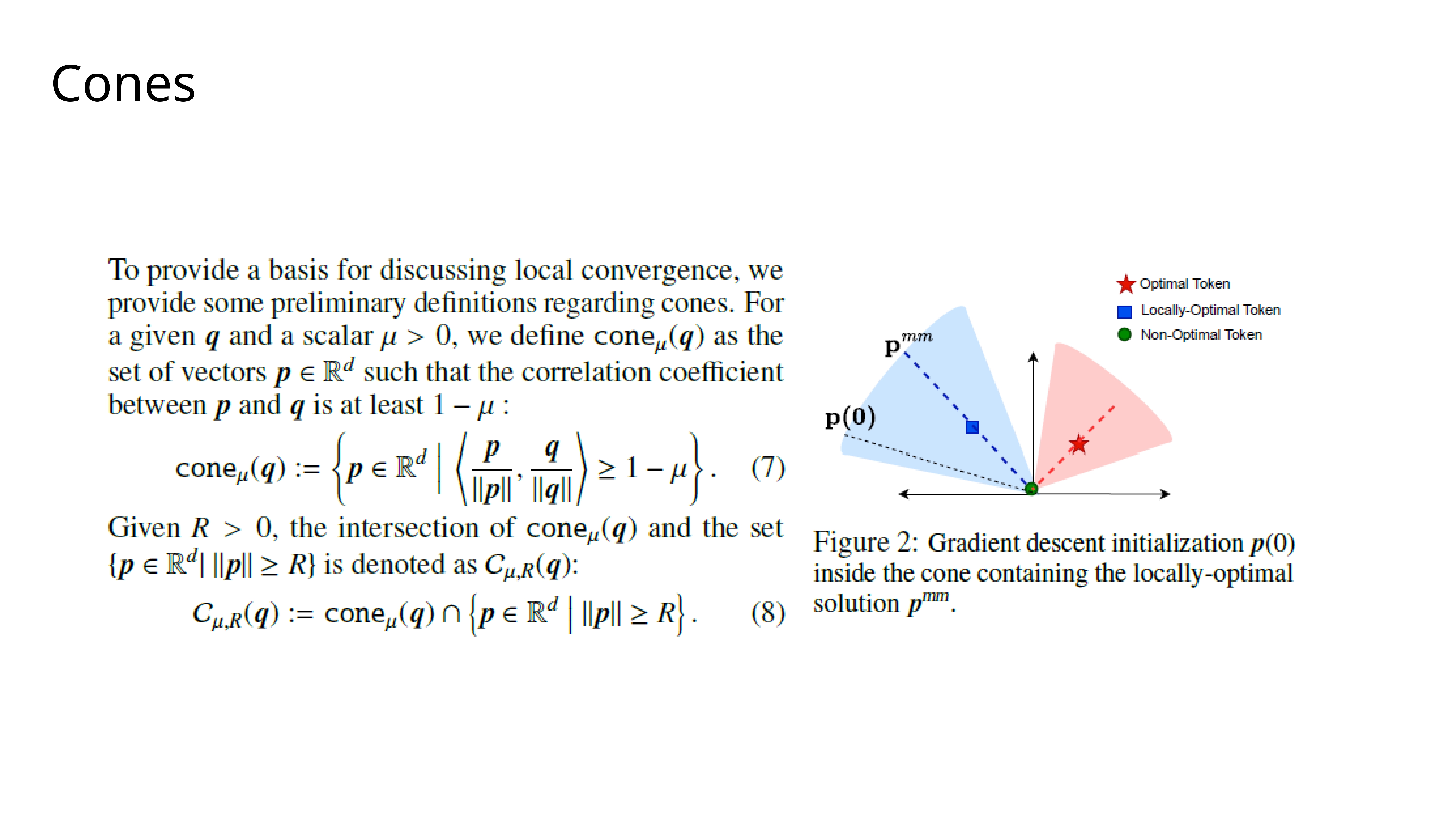
To talk about local convergence, we introduce the geometric concept of a cone. A cone around a direction q is simply the set of all vectors that are “close” in angle to q. The diagram illustrates an initialization p(0) that lies within the cone of an LMM direction p^mm.

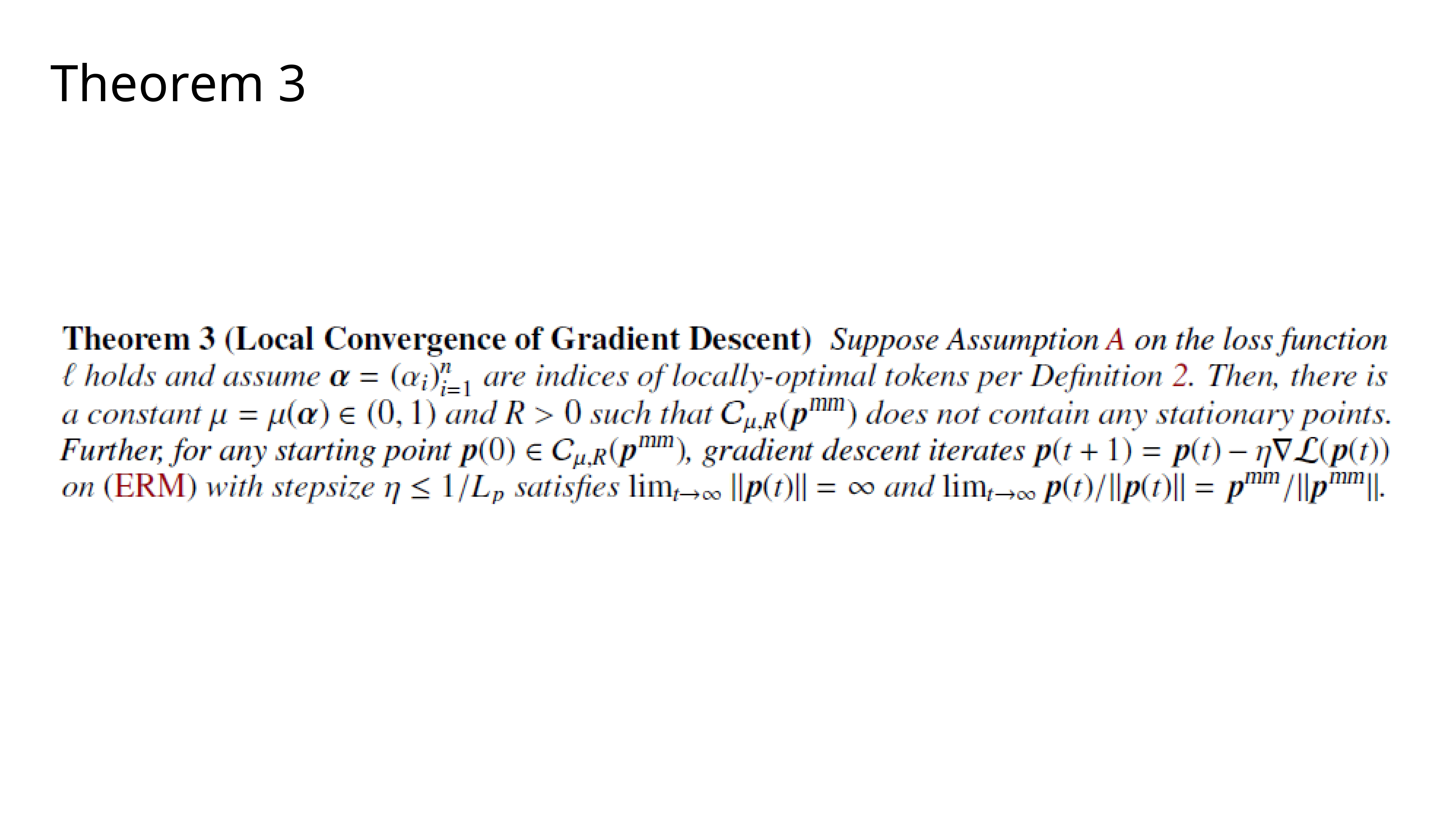
Theorem 3 formalizes local convergence. It states that if you initialize the gradient descent p(0) within the cone of an LMM direction, the optimization will stay within that cone and ultimately converge to that specific LMM direction.

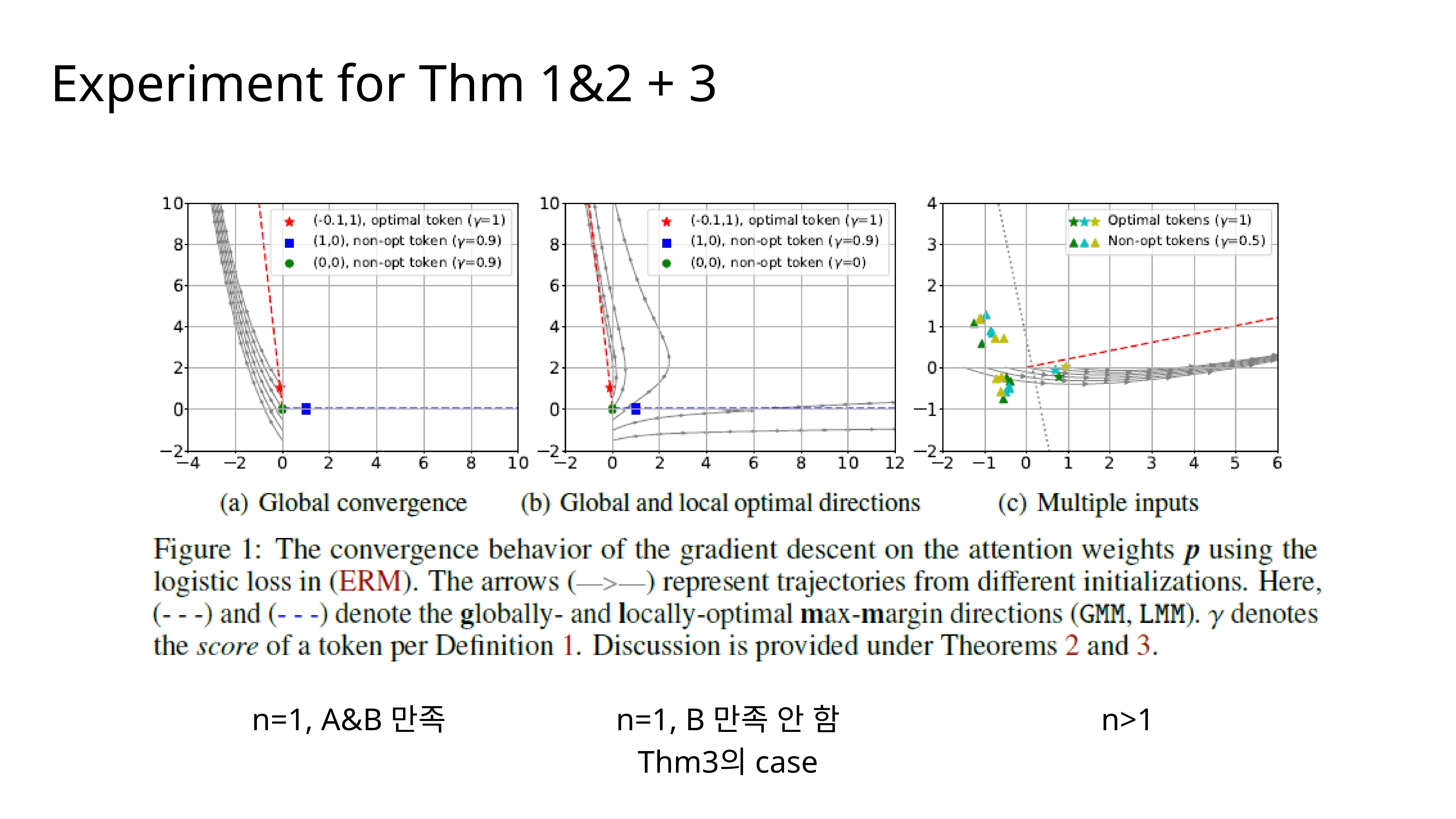
Looking back at our experiment in Figure (b), we can now understand it better through Theorem 3. The trajectories that don’t find the global optimum are the ones that were initialized inside the cone of the locally-optimal solution (the blue square), and as the theorem predicts, they converge to it.

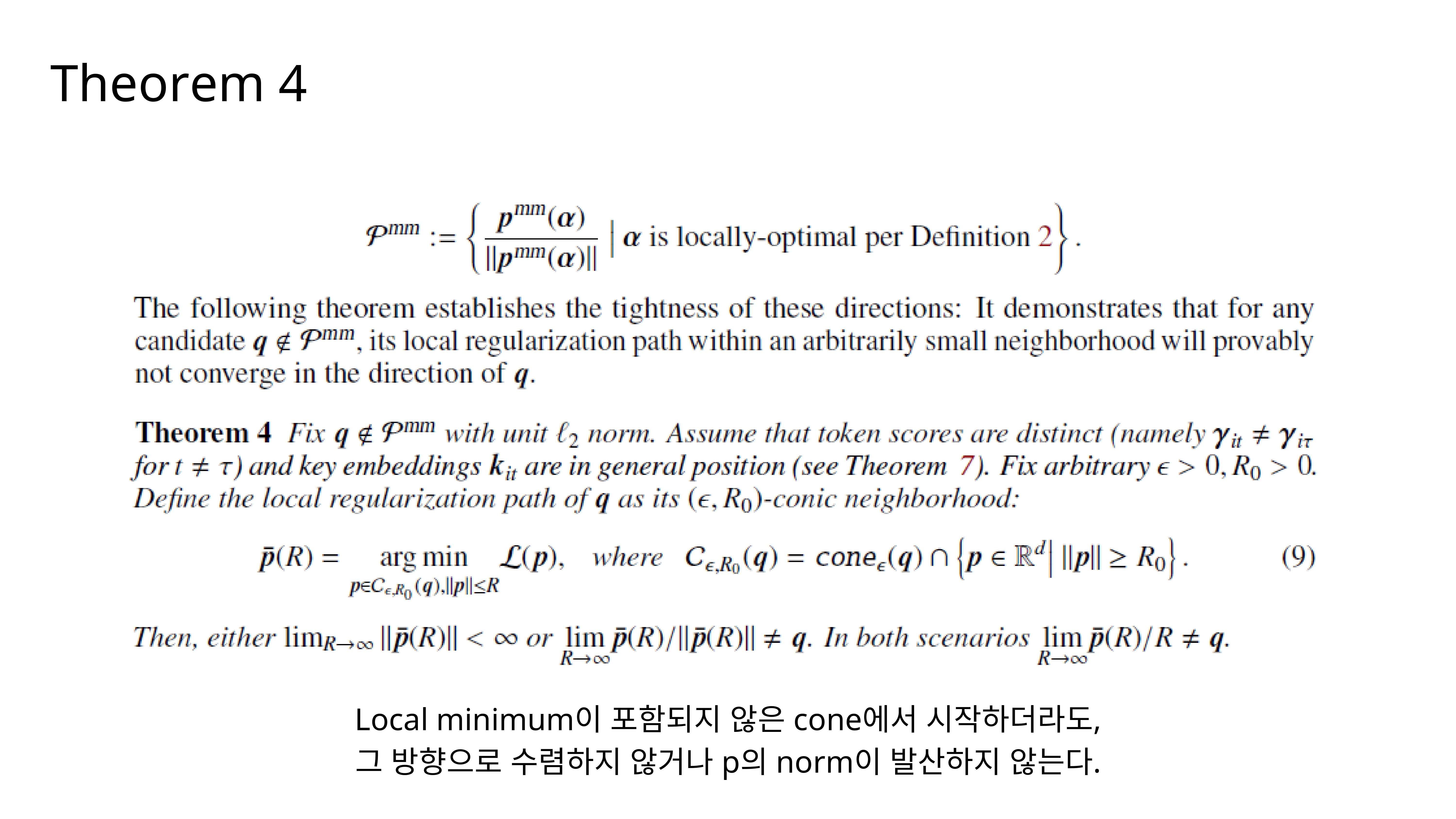
Theorem 4 provides a tightness guarantee. It essentially says that the LMM directions are the only stable convergence points. If you start in any direction q that is not an LMM direction, the optimization path will eventually move away from q.

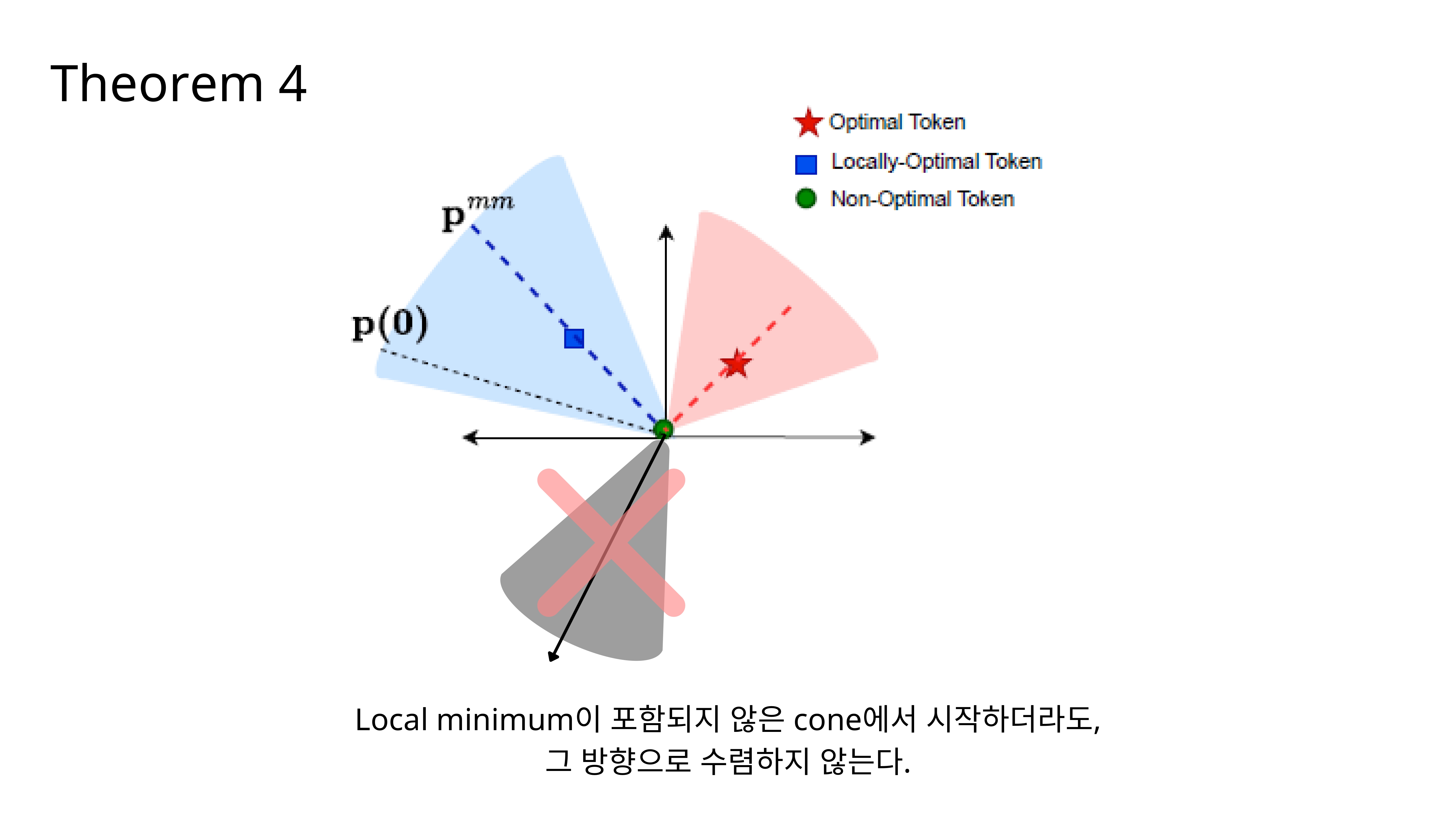
This diagram illustrates Theorem 4. If our initial parameter p(0) is in a cone (the grey one) that does not contain any LMM or GMM direction, the optimization process will not converge in that direction. It is implicitly forced to seek out one of the valid max-margin solutions.

To summarize the first half: we’ve shown that when training only the attention parameter p, the implicit bias of gradient descent drives the solution towards a hard-margin SVM that separates tokens. Now, what happens if we also learn the prediction head v at the same time?

This leads to the second part of our analysis: the joint convergence of the prediction head v and the attention weights p.

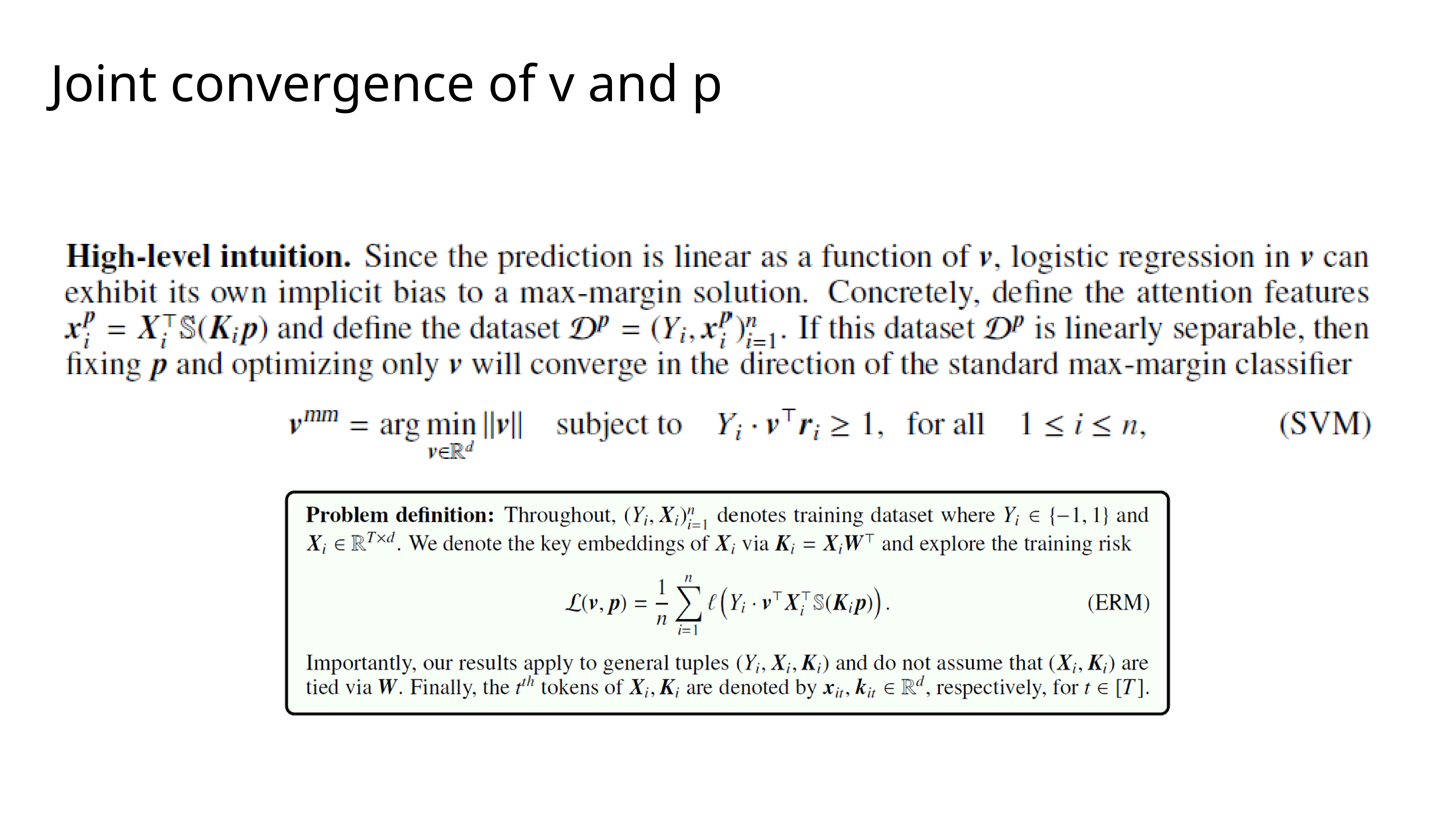
The high-level intuition is that the model is linear in v, so the optimization with respect to v also has an implicit bias towards a standard max-margin classifier solution. The features for this classifier, x_i^p, are the outputs of the attention layer.

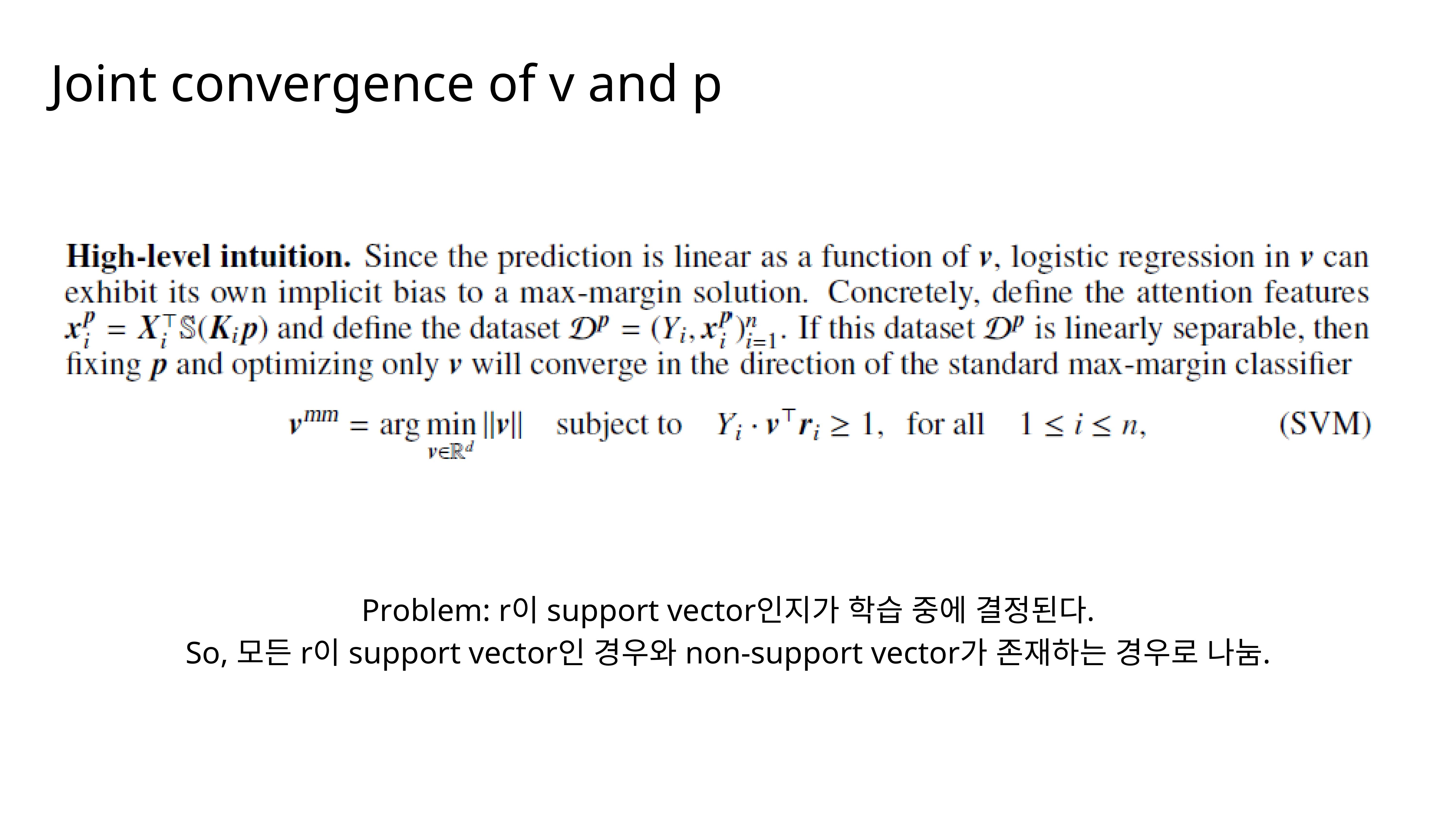
The challenge here is that the features r that v sees are determined by p, which itself is changing during training. This creates a coupled dynamic. We analyze this by separating the problem into cases based on whether the selected features are support vectors for the v-classifier or not.

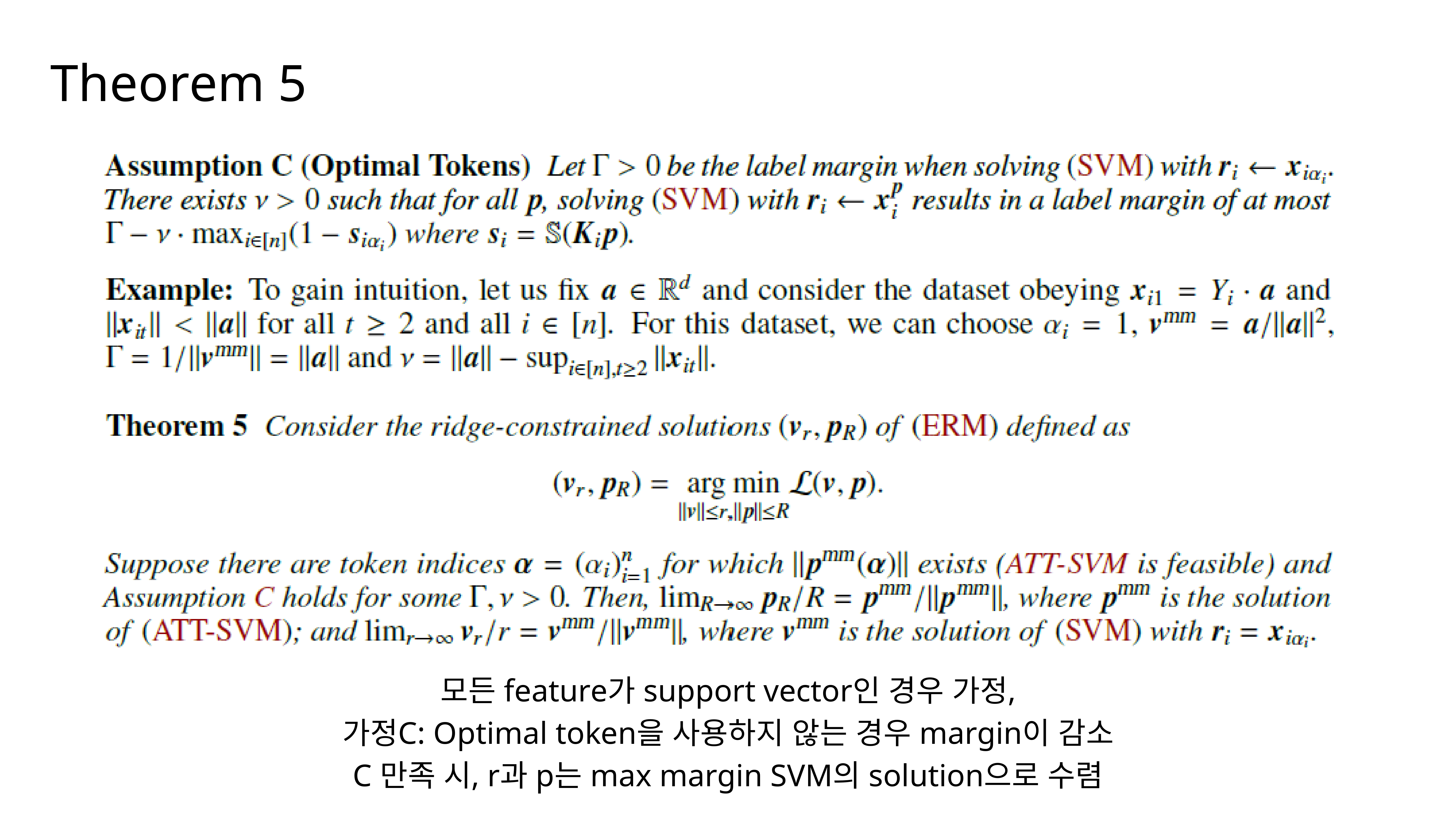
Theorem 5 addresses the case where we assume the selected tokens are all support vectors. We introduce Assumption C, which formalizes that if the attention doesn’t perfectly select the optimal token, the classification margin for v shrinks. Under this assumption, we find that v converges to the direction of a standard SVM solution, and p converges to the direction of our ATT-SVM solution.

This raises a natural question: Does every selected token really need to be a support vector, sitting right on the margin? That seems like a very strict condition. Intuitively, for the data points that are not support vectors, we don’t need to maximize their margin. We just need to make sure they are on the correct side of the decision boundary. This allows us to define a “relaxed” version of our ATT-SVM problem.

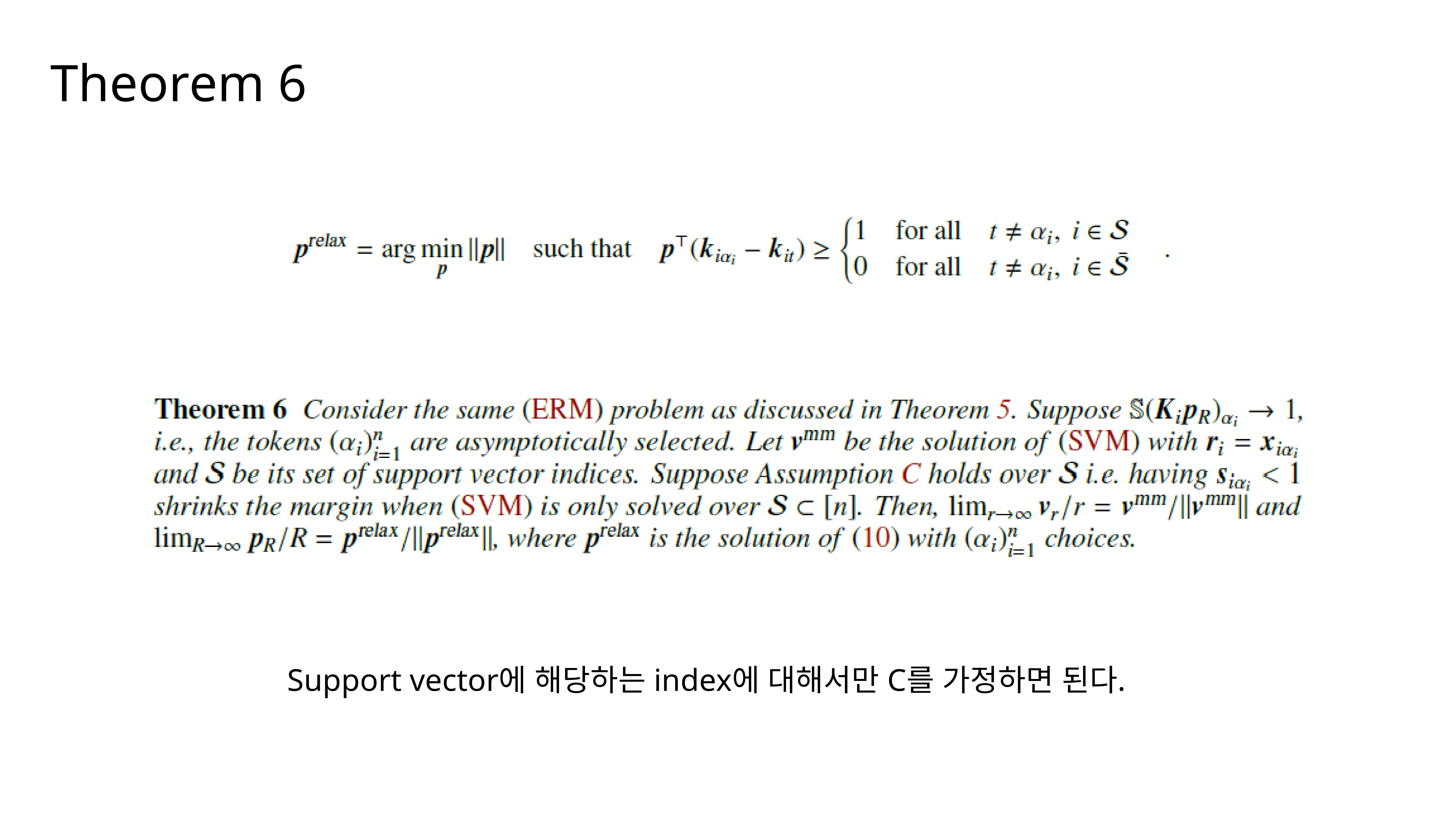
Theorem 6 presents this more general result. The ATT-SVM problem is relaxed: for tokens corresponding to support vectors (i ∈ S), we require a margin of 1, but for non-support vectors (i ∈ S-bar), we only require a margin of 0 (correct classification). We only need Assumption C to hold for the support vectors. The result is that v still converges to the max-margin v^mm, and p converges to the solution of this new, relaxed SVM problem, p^relax.

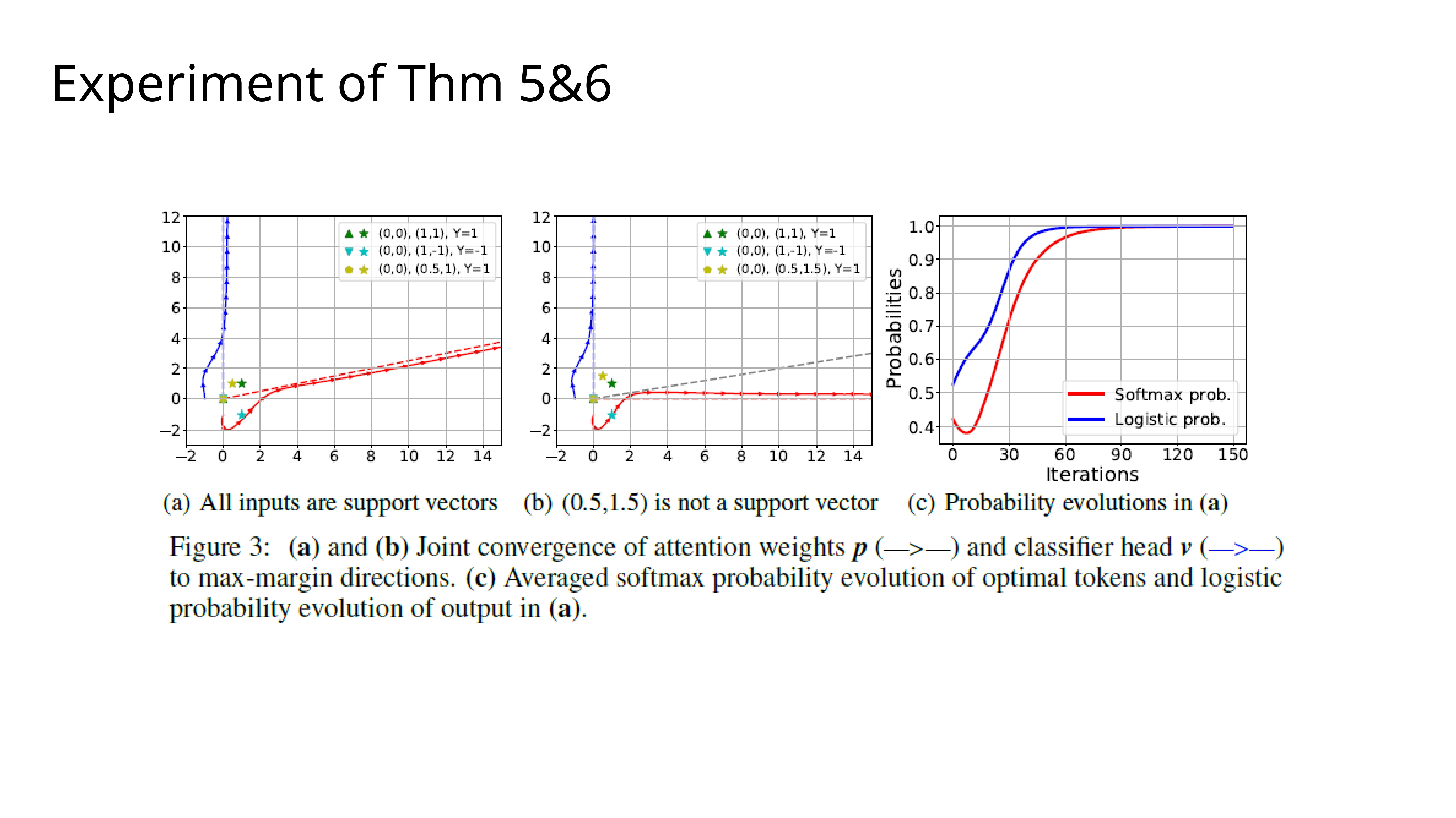
We ran experiments for this joint convergence case as well. The plots show the trajectories for the attention weights p and the classifier head v. Plot (a) shows a case aligning with Theorem 5, where all inputs are support vectors. Plot (b) shows a case for Theorem 6, where one input is not a support vector. Plot (c) shows that the softmax probability for the optimal token quickly goes to 1, confirming that the attention is learning to select specific tokens as predicted.

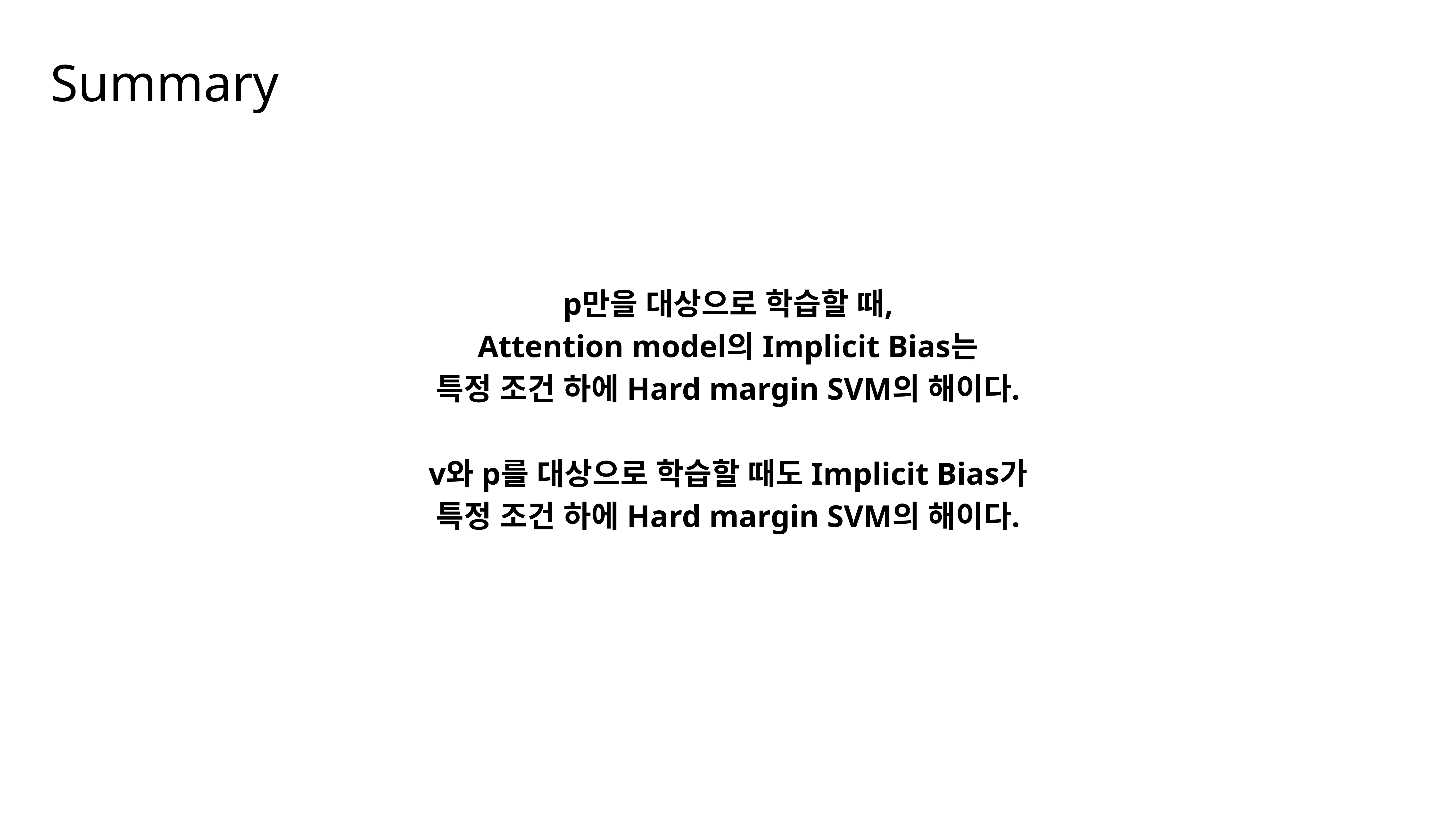
So, to summarize the entire theoretical part: Whether we train the attention weights p alone or jointly with the classifier head v, the implicit bias of the optimization consistently pushes the model towards a hard-margin SVM solution. This provides a strong theoretical explanation for why attention learns to become sparse and focus on the most discriminative tokens.

Finally, let’s look at a few more experiments to see these principles in action on more complex tasks.

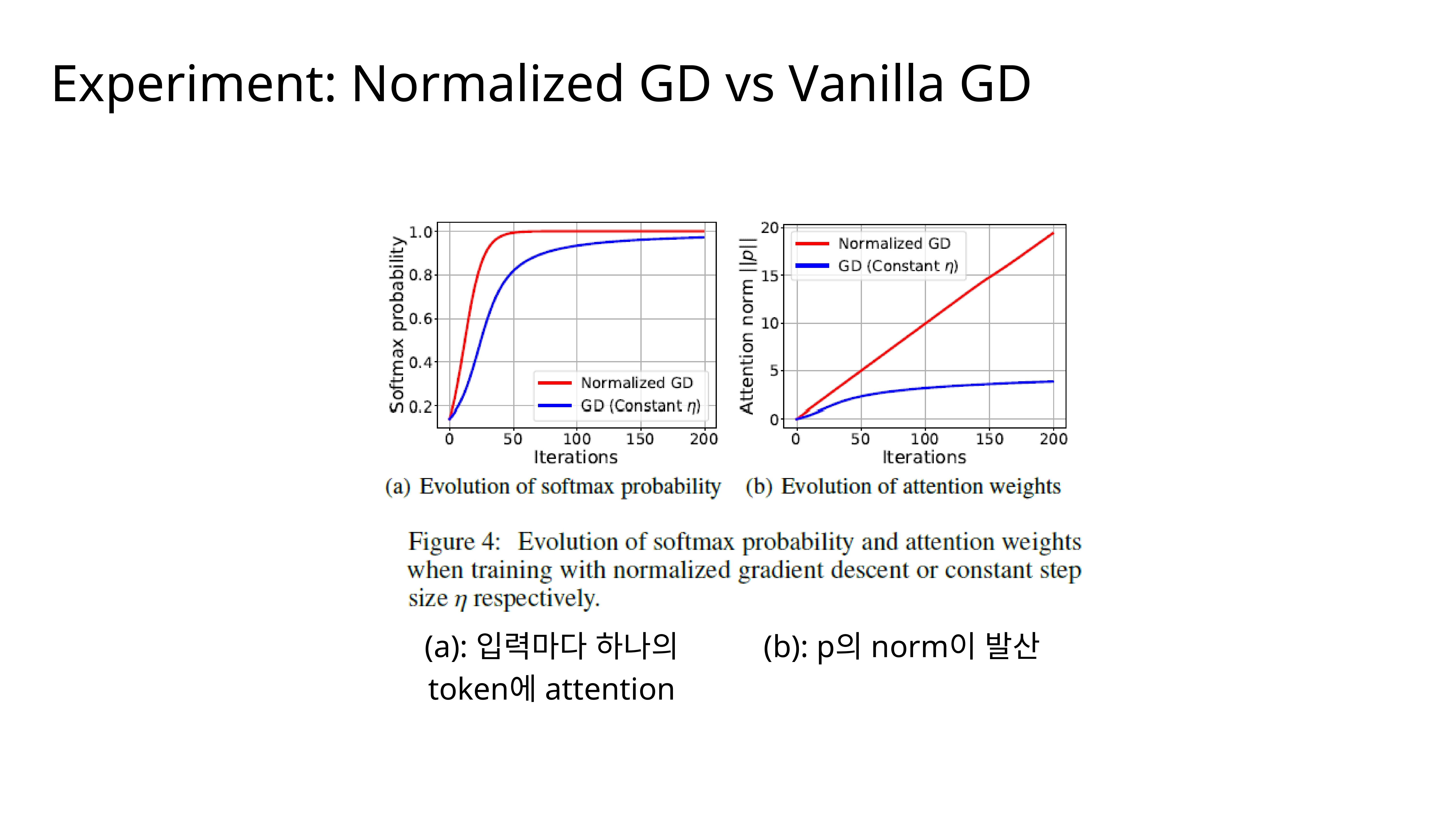
This slide provides an experimental comparison between Normalized Gradient Descent (GD) and Vanilla GD, validating the paper’s theory. Plot (a) shows that while both methods learn to focus on a single token (softmax probability approaches 1.0), Normalized GD achieves this sparse attention much faster. Plot (b) demonstrates a key theoretical prediction: the norm of the attention weights ||p|| diverges (grows linearly without bound) when using Normalized GD. This behavior is characteristic of an optimization process seeking a max-margin solution.

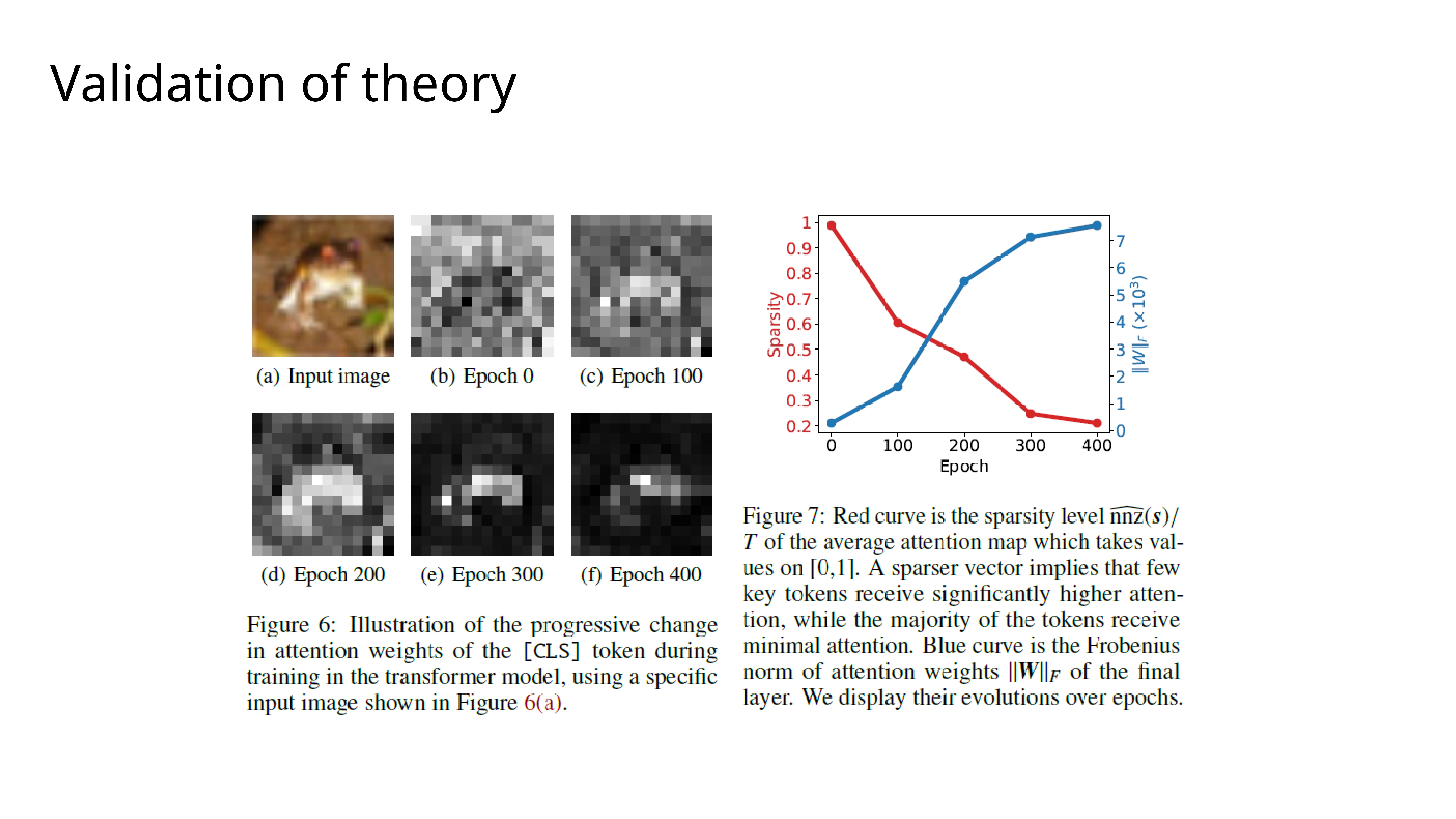
Here, we trained a vision transformer on an image classification task. Figure 7 shows that as training progresses over epochs, the sparsity of the attention map increases (red curve goes down), meaning the model learns to focus on fewer, more important image patches. At the same time, the norm of the attention weights ||W|| steadily increases (blue curve), which is exactly what our theory predicts will happen as the solution converges towards an infinite-norm, max-margin boundary. The images in Figure 6 visually show this focusing effect over time.

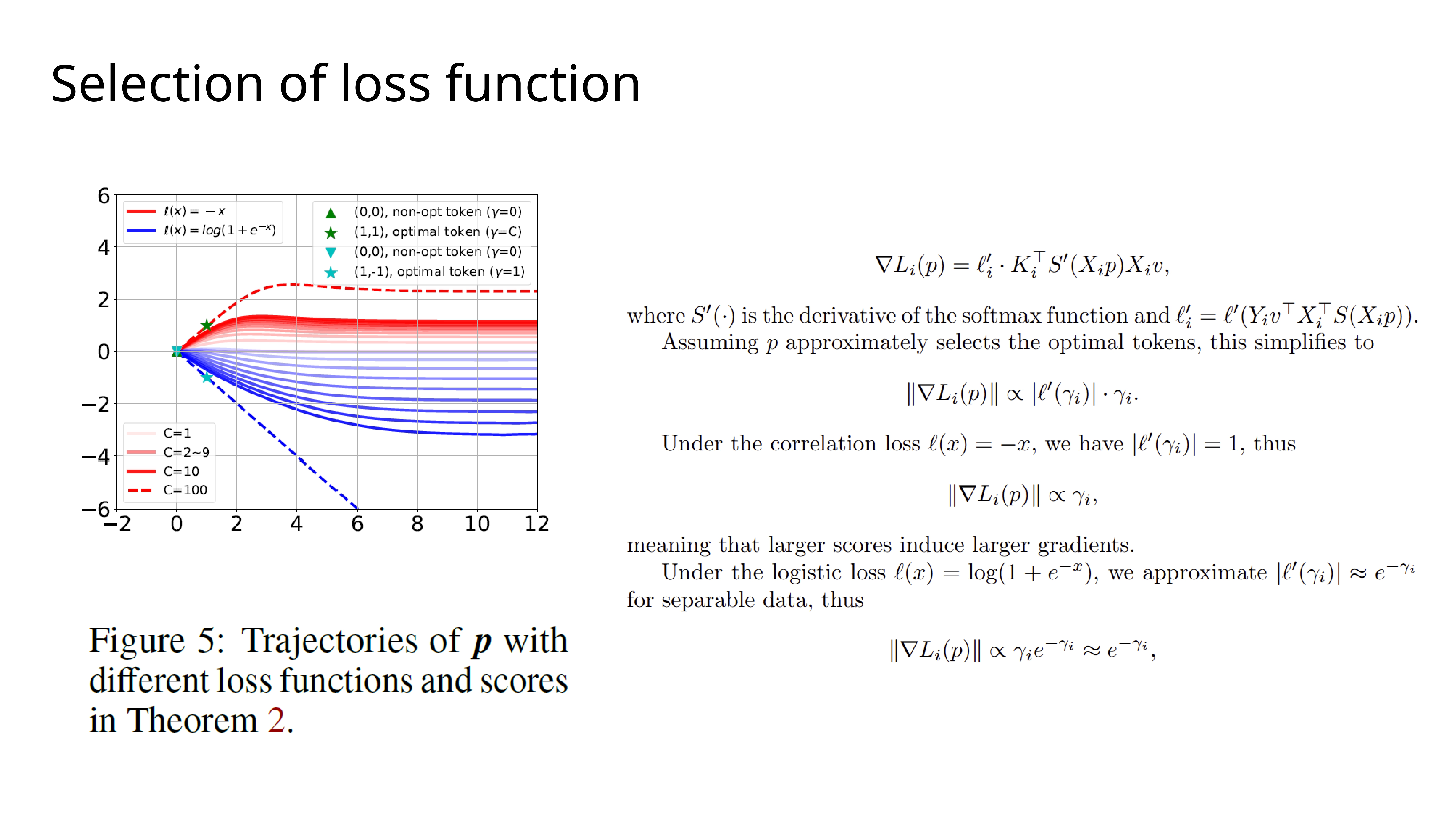
This final experiment shows how the choice of loss function affects the dynamics. We compare a correlation loss (l(x) = -x) with the logistic loss. The gradient’s magnitude depends on the token’s score γ differently for each loss. For correlation loss, larger scores get larger gradients, while for logistic loss, the gradient is largest for scores near zero. This results in different trajectories, but as you can see, both are ultimately guided by the same underlying max-margin principle, pushing towards a separating hyperplane.