This is a foundational paper from NIPS 1994 that introduced an idea that has become highly relevant again in the modern deep learning era: the connection between the geometry of the loss landscape and a model’s ability to generalize.
The core idea is simple yet powerful: instead of just finding the lowest point of the error function (the minimum), we should actively search for wide, flat regions. A model that corresponds to a flat minimum is less sensitive to small changes in its weights, which often translates to better performance on unseen data.

This is the title slide for my presentation on “Simplifying neural nets by discovering flat minima,” which I prepared for our lab meeting.

First, let’s credit the authors: Sepp Hochreiter and Jürgen Schmidhuber. As you can see, this is a fairly old paper, but its insights are timeless and arguably more important than ever given the flood of modern research. The key question is, what can we learn from it today?

Here are the authors of the paper. This work was originally presented at the NIPS 1994 conference (now known as NeurIPS).

This quote from the authors perfectly captures the paper’s central thesis: “Find wide, not sharp, minima - and your network generalizes for free.” It elegantly states that good generalization is a natural consequence of the shape of the solution space we find.

My presentation is structured into three main parts: First, the motivation for why we need a new approach. Second, a deeper dive into the core idea of flat minima. And finally, the specific algorithm they developed to find them.

So, let’s start with the motivation. Why was this research necessary?
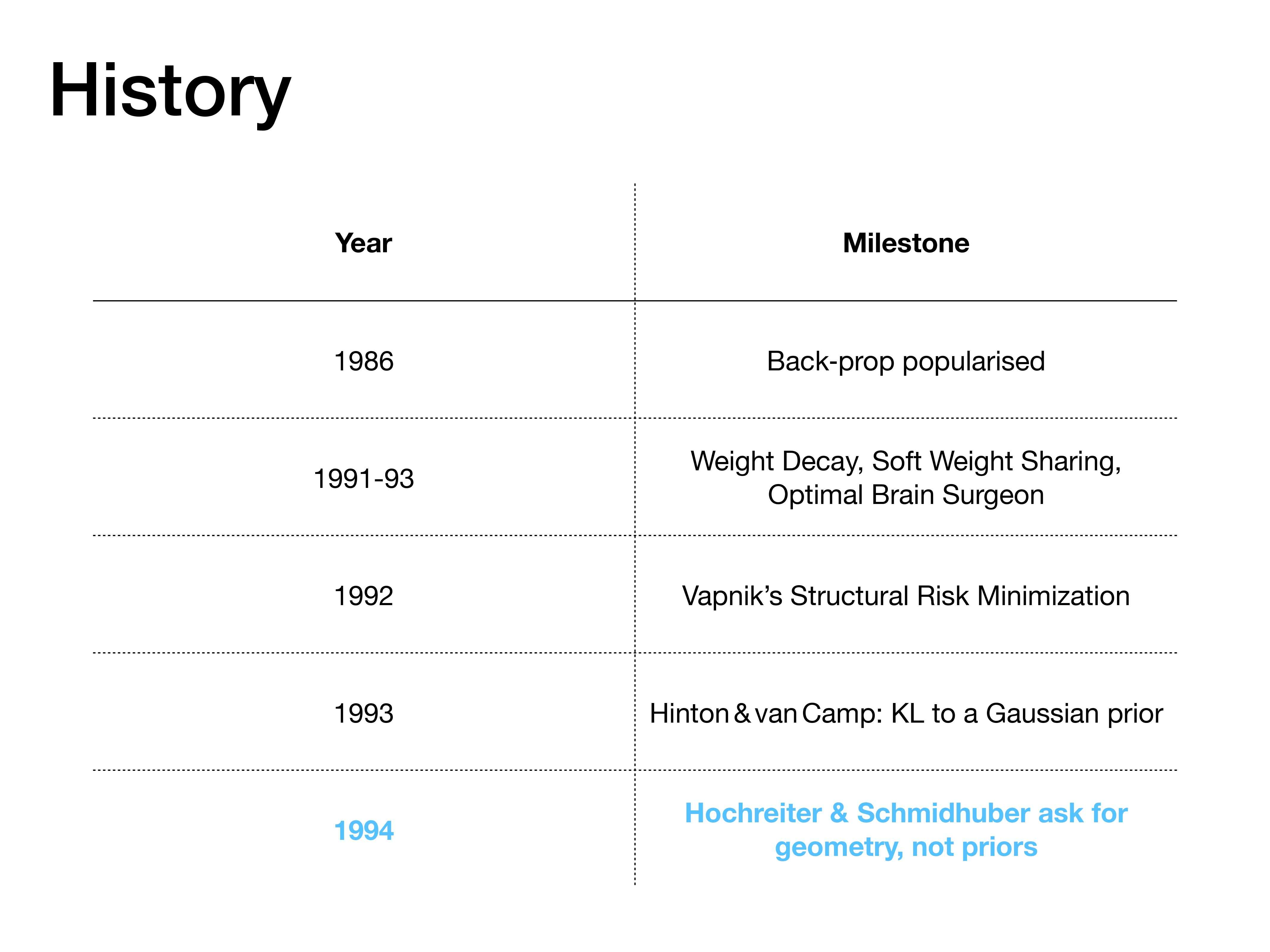
To understand the paper’s contribution, it helps to look at the historical context. In the years leading up to 1994, popular techniques for improving generalization like Weight Decay and Optimal Brain Surgeon were based on making assumptions about the network’s weights (so-called “priors”). This paper marked a shift, arguing that we should focus on the geometry of the error surface rather than imposing assumptions about the weights themselves.
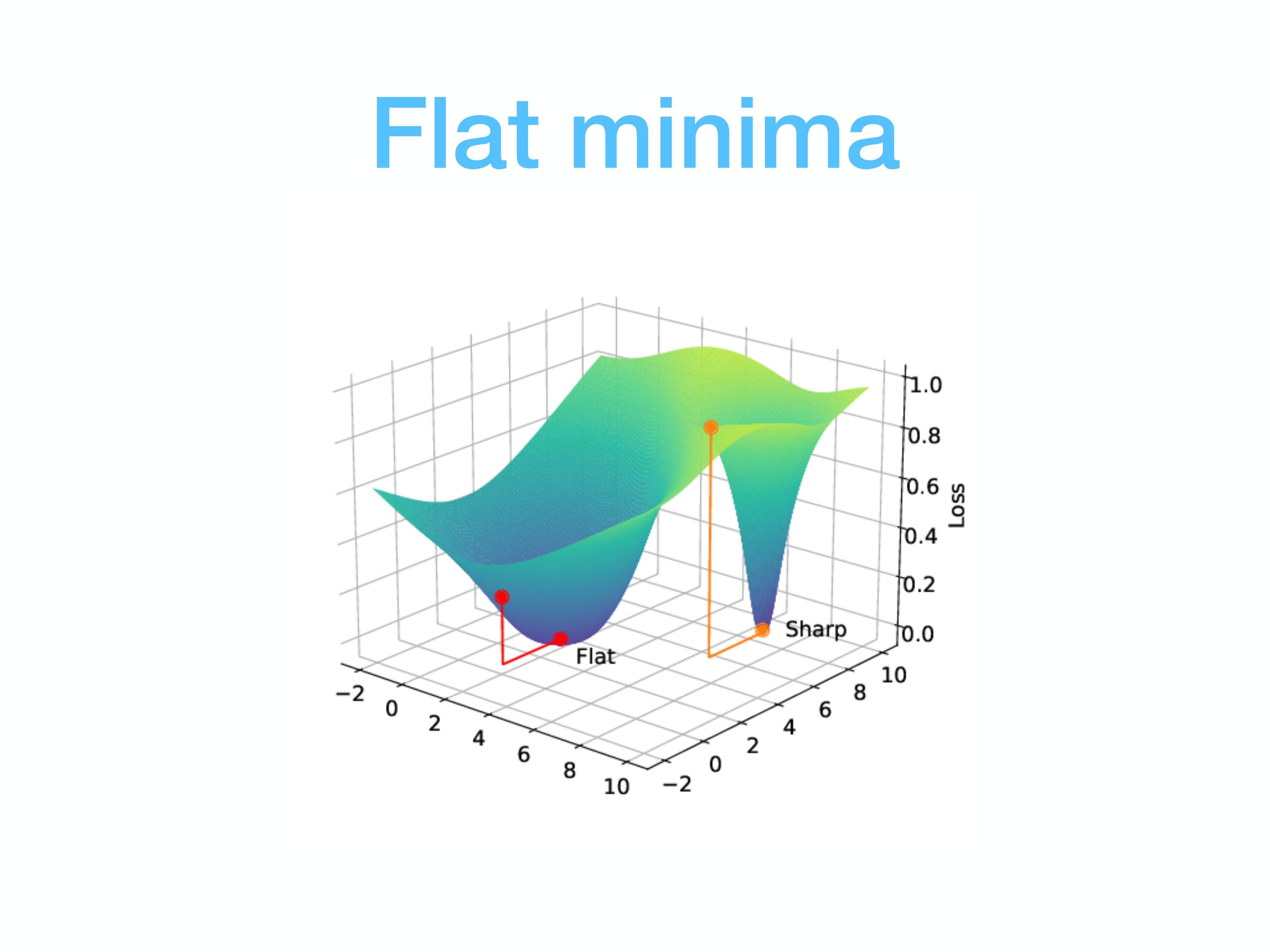
This 3D plot illustrates the core concept perfectly. On the right, we see a “sharp” minimum. While the loss is low at the very bottom, a small perturbation to the weights can cause a dramatic increase in loss. On the left, we have a “flat” minimum. Here, the loss remains low across a large connected region of the weight space. The hypothesis is that solutions in these flat regions are more robust and generalize better.
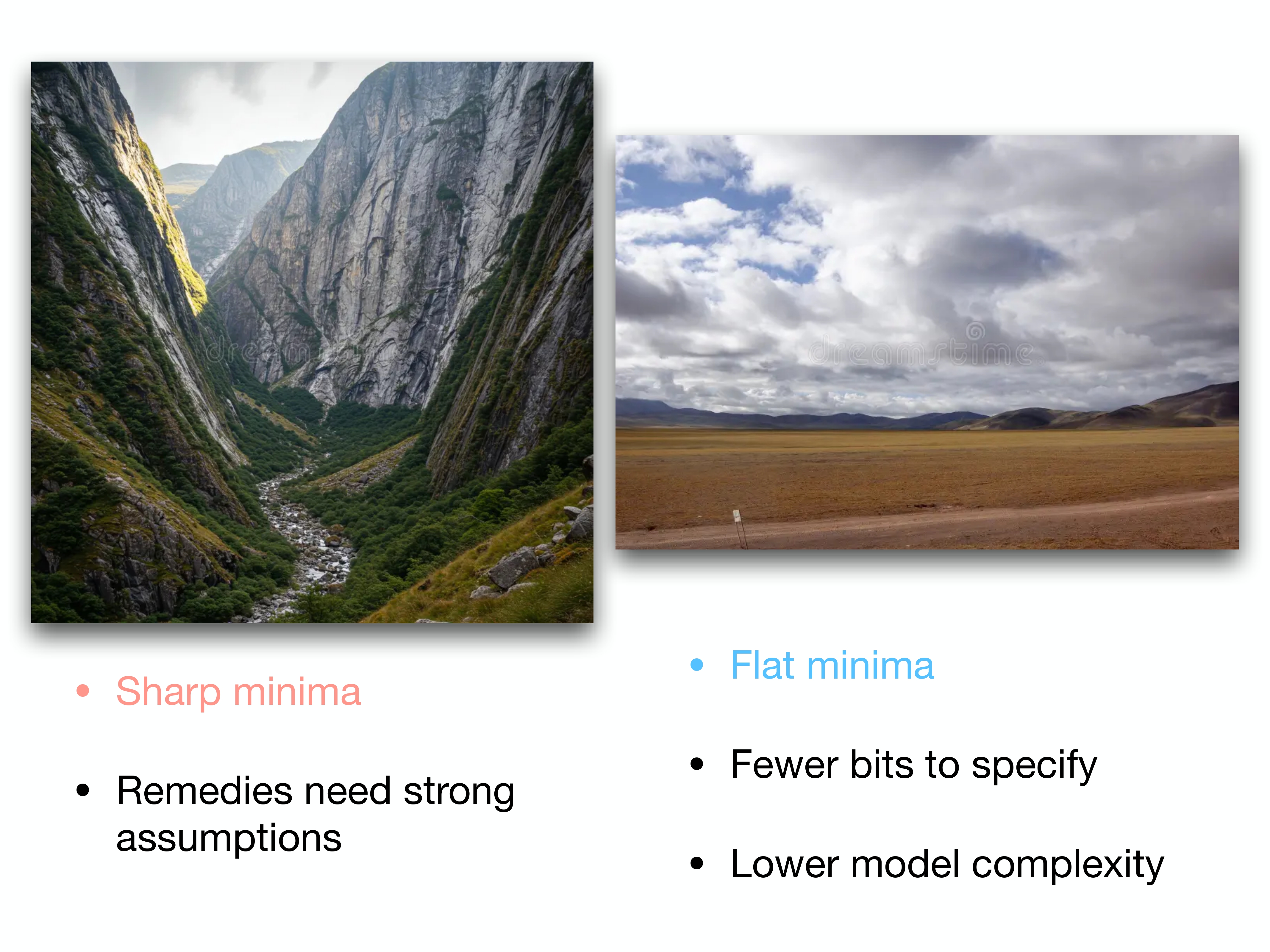
Here’s a simple visual analogy. A sharp minimum is like a deep, narrow canyon. It’s difficult to land exactly at the bottom, and any small error puts you high up on the canyon walls. A flat minimum is like a wide, open valley. It’s much easier to find a good spot, and moving around a little doesn’t drastically change your altitude (or your model’s error). This robustness is linked to lower model complexity.
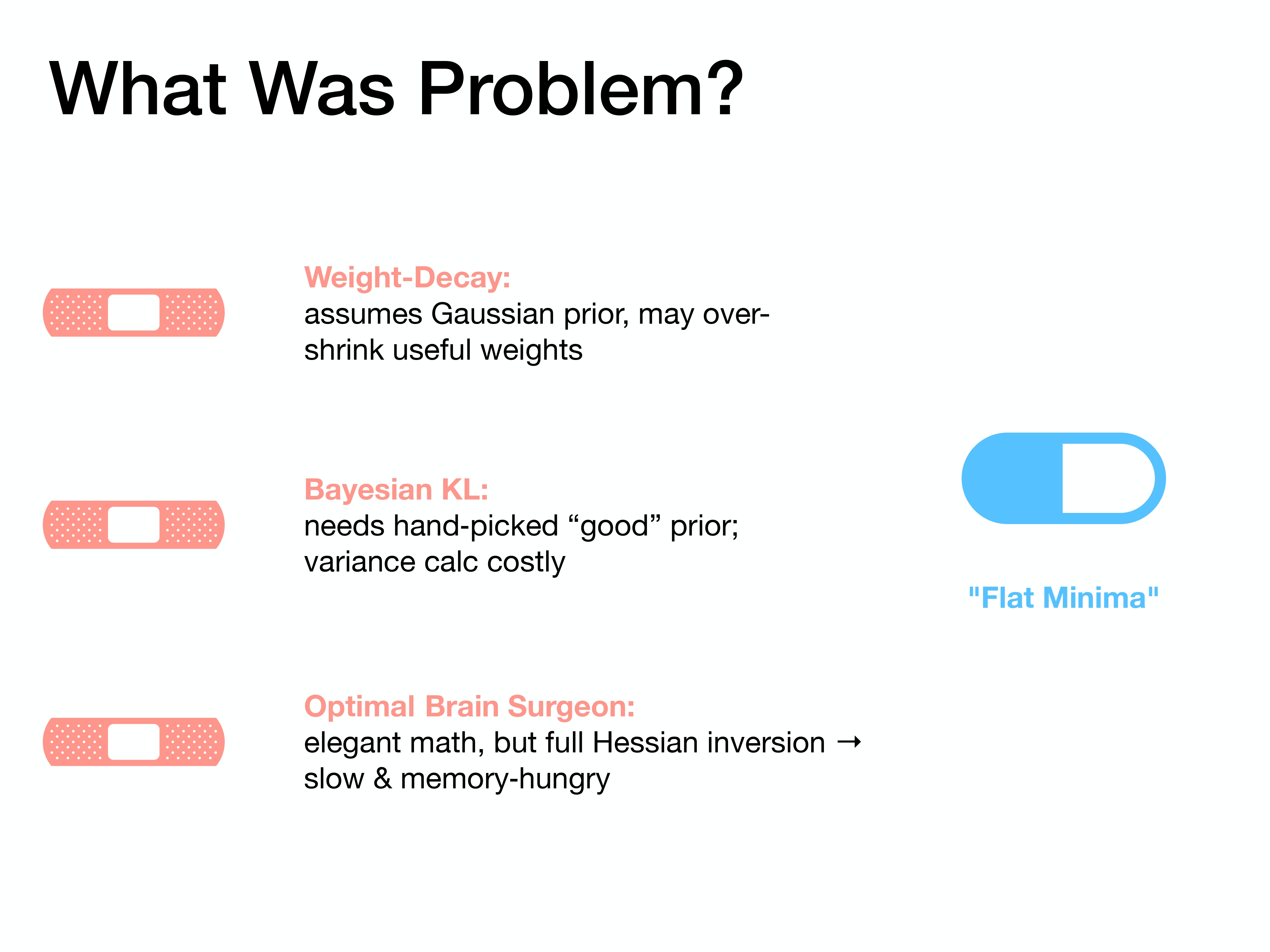
So, what was wrong with the existing methods? Weight-Decay, for instance, assumes a Gaussian prior and can sometimes shrink important weights too aggressively. Bayesian methods require you to hand-pick a “good” prior distribution. And methods like Optimal Brain Surgeon, while elegant, were very slow and memory-intensive because they required inverting the full Hessian matrix.
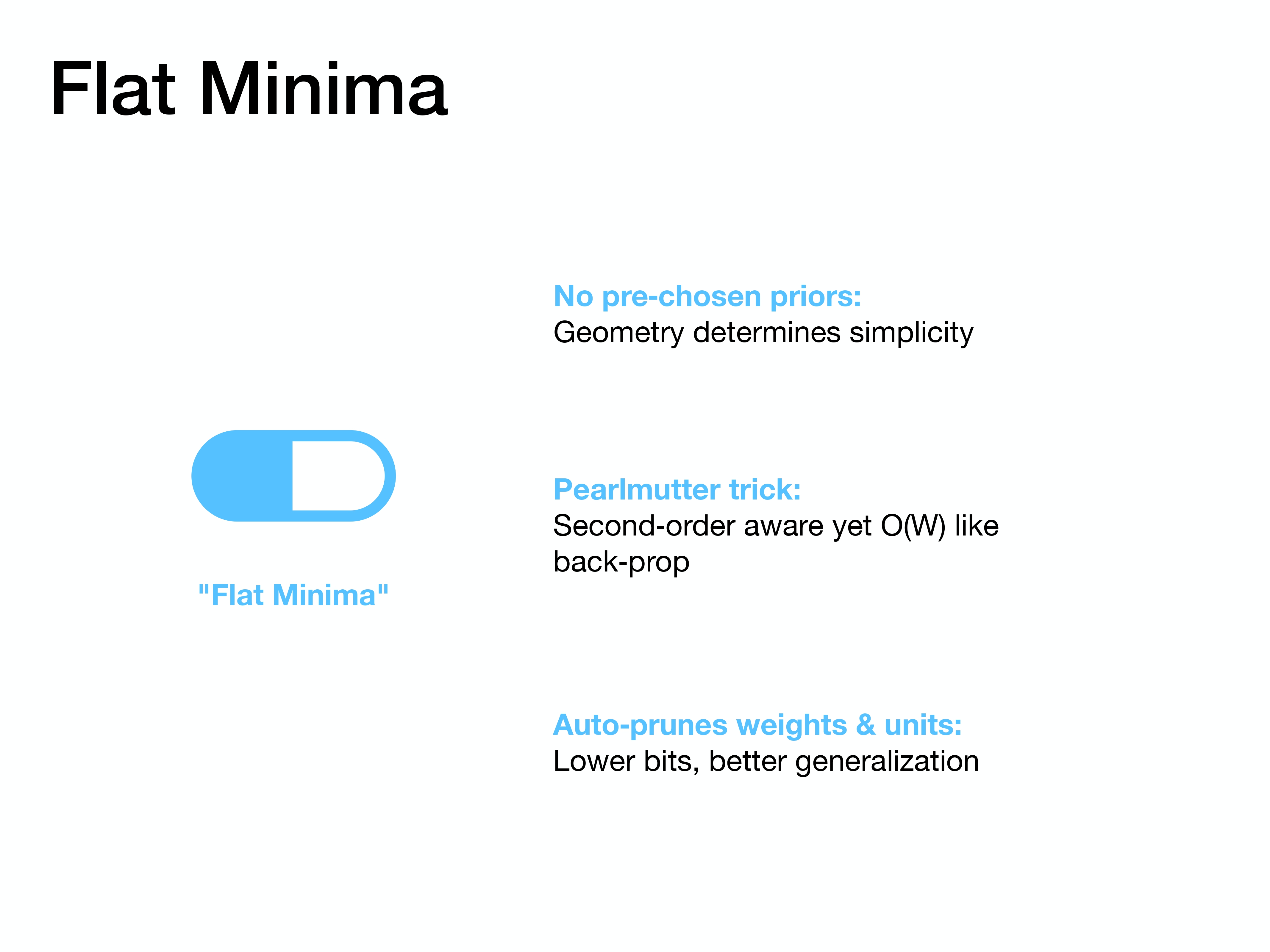
The “Flat Minima” approach offers solutions to these problems. First, it doesn’t require any pre-chosen priors; the geometry of the solution space itself defines what a “simple” model is. Second, it uses a clever computational method that makes it aware of second-order information but keeps the complexity on the same order as standard back-propagation. Finally, this process naturally prunes unnecessary weights, leading to a simpler model.

Now, let’s formalize the problem by defining the tasks and architectures this method applies to.
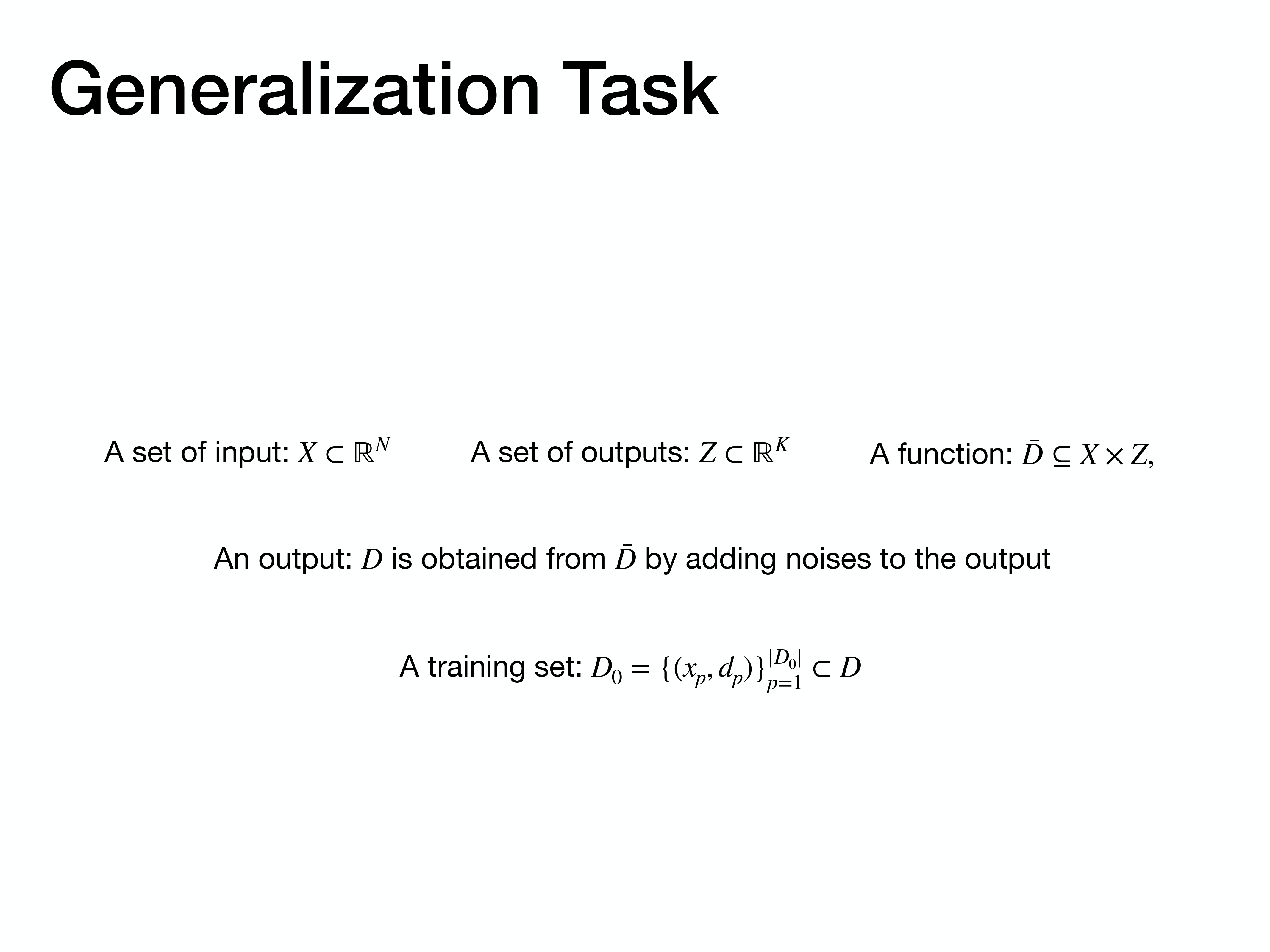
The basic setup is a standard supervised learning problem. We have a set of inputs and outputs, and our training data consists of input-output pairs where the outputs have been perturbed by some noise.
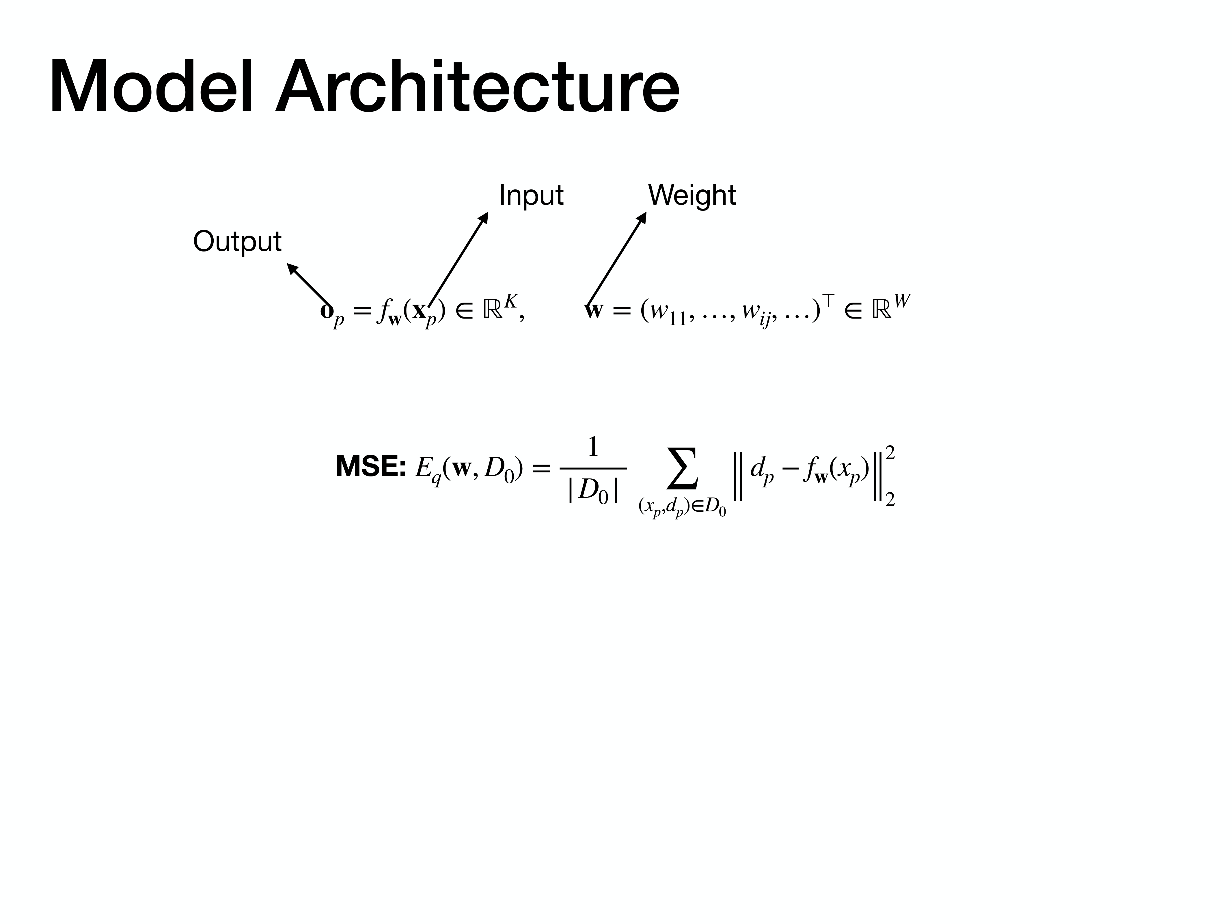
The model is a neural network, represented by the function $f_w(x_p)$, which takes an input $x_p$ and produces an output, parameterized by a set of weights $W$. We measure its performance on the training set using the Mean Squared Error (MSE).
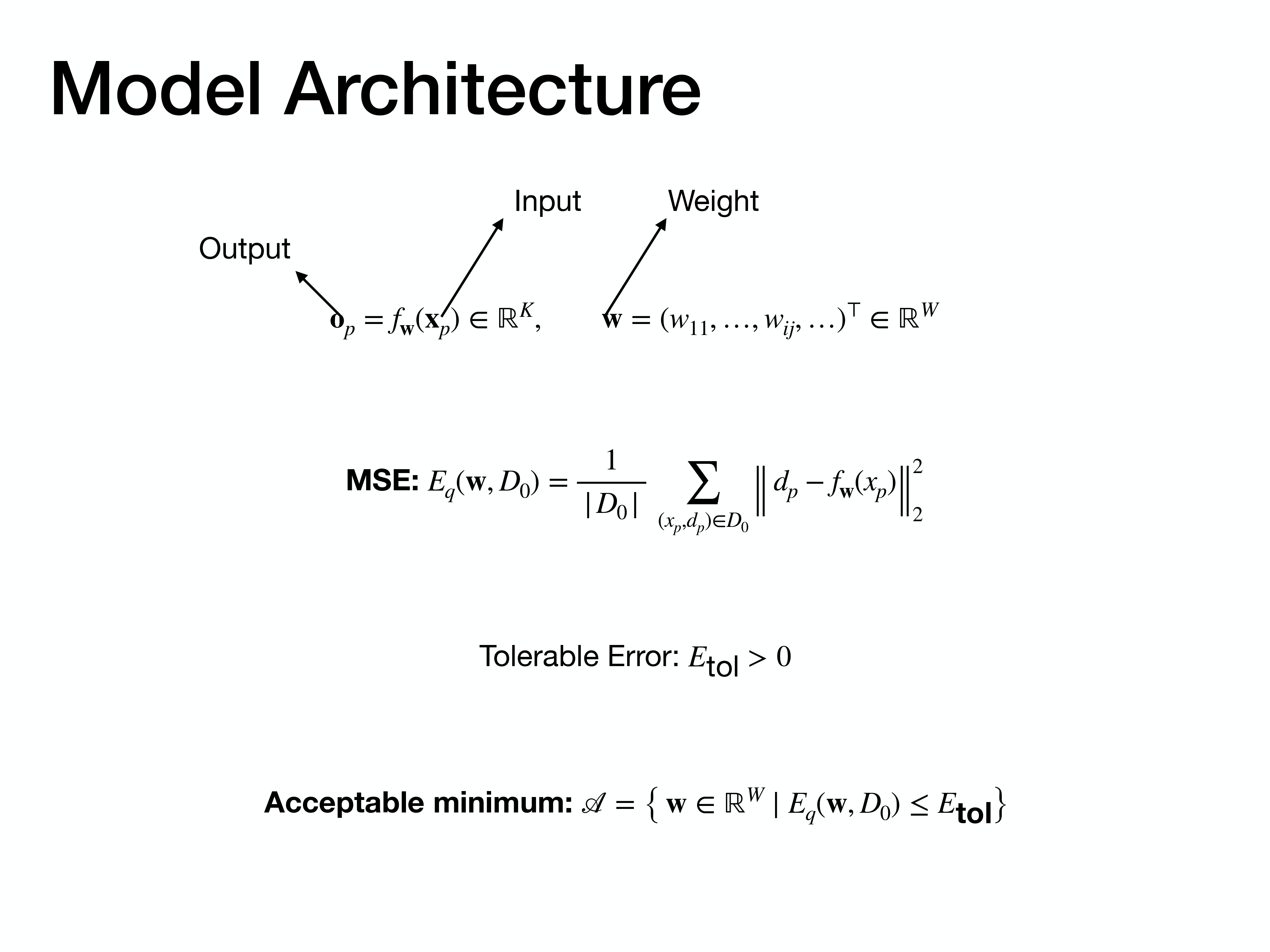
Building on that, we can define the set of “acceptable” solutions. Given a tolerable error level, $E_{tol}$, the acceptable minimum is the entire set of weight vectors
wfor which the training MSE is less than or equal to this tolerance.
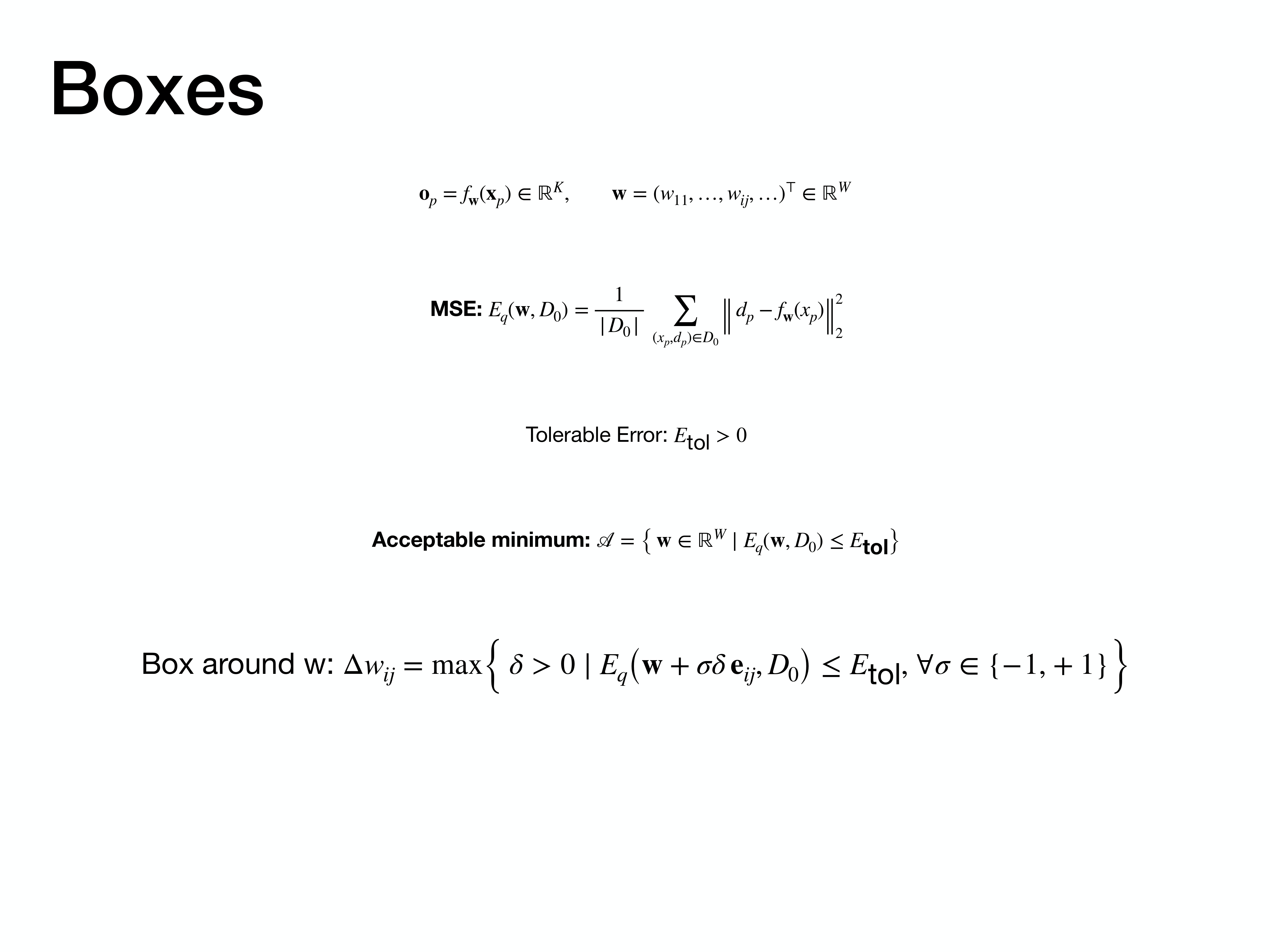
Now we get to the core of the algorithm’s construction. For a given weight vector
w, we define a “box” around it. For each individual weight $w_{ij}$, we find the maximum amount $\delta$ it can be perturbed before the training error exceeds our tolerance $E_{tol}$. This gives us an interval $\Delta w_{ij}$ for each weight.
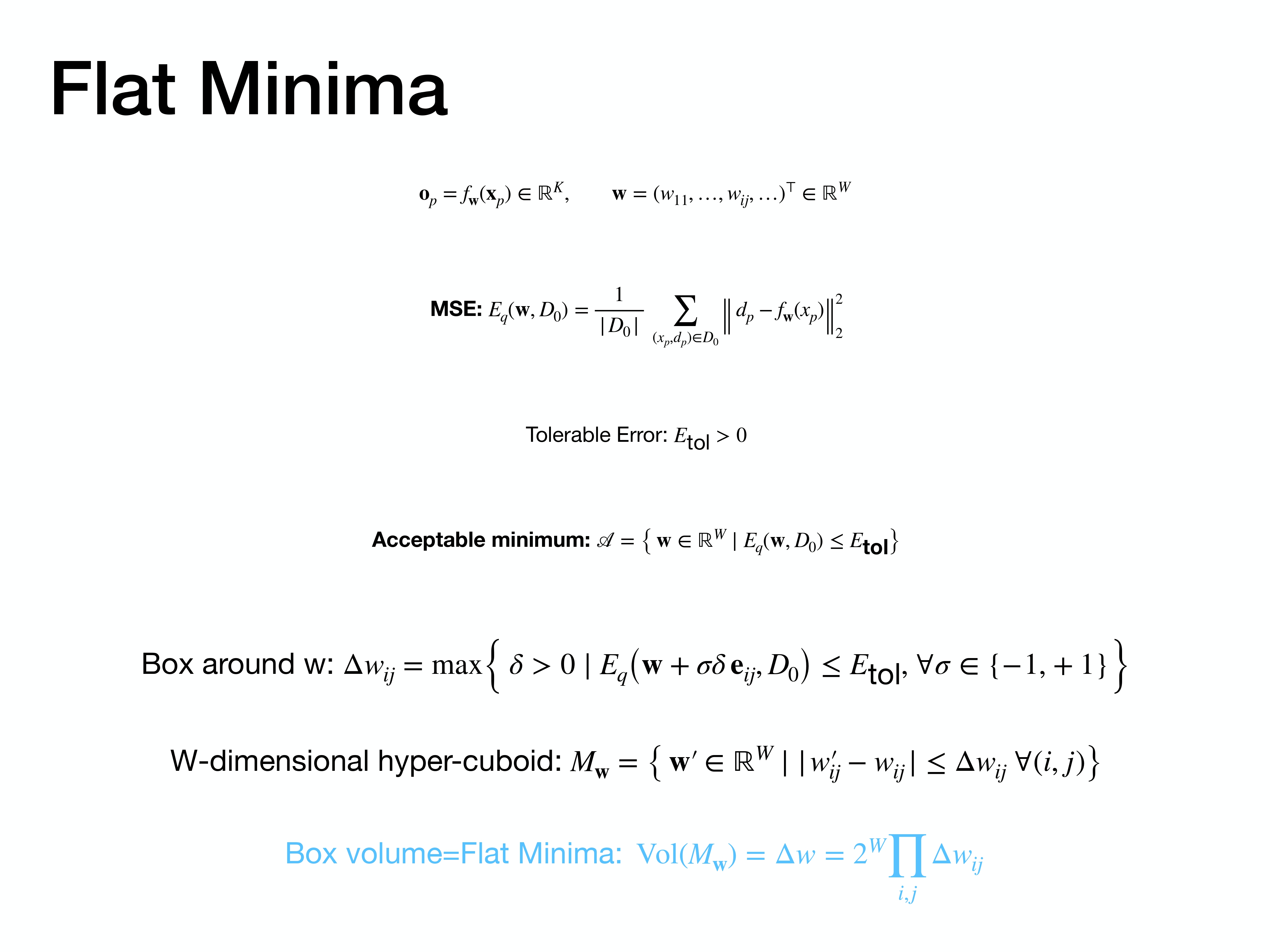
These intervals for all the weights combine to form a high-dimensional hyper-cuboid in the weight space. The paper defines the “Flat Minima” as the volume of this box. The larger the volume, the flatter the minimum, and the more robust the solution.

So, how do we actually find these large-volume minima? That brings us to the algorithm itself.
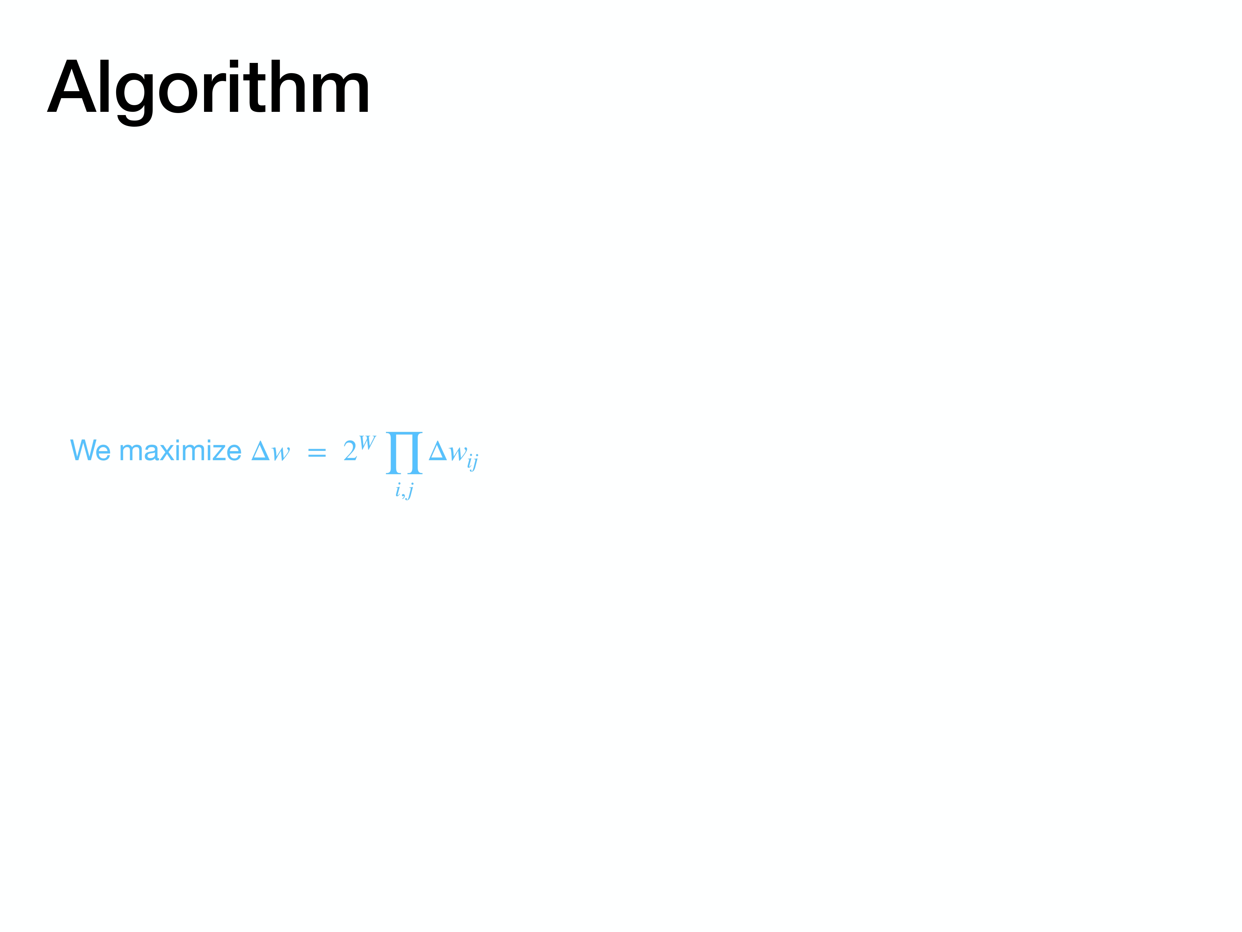
The main objective of the algorithm is to maximize the volume of the box in weight space, which is represented as $\Delta w$. A larger volume signifies a flatter, more desirable minimum.
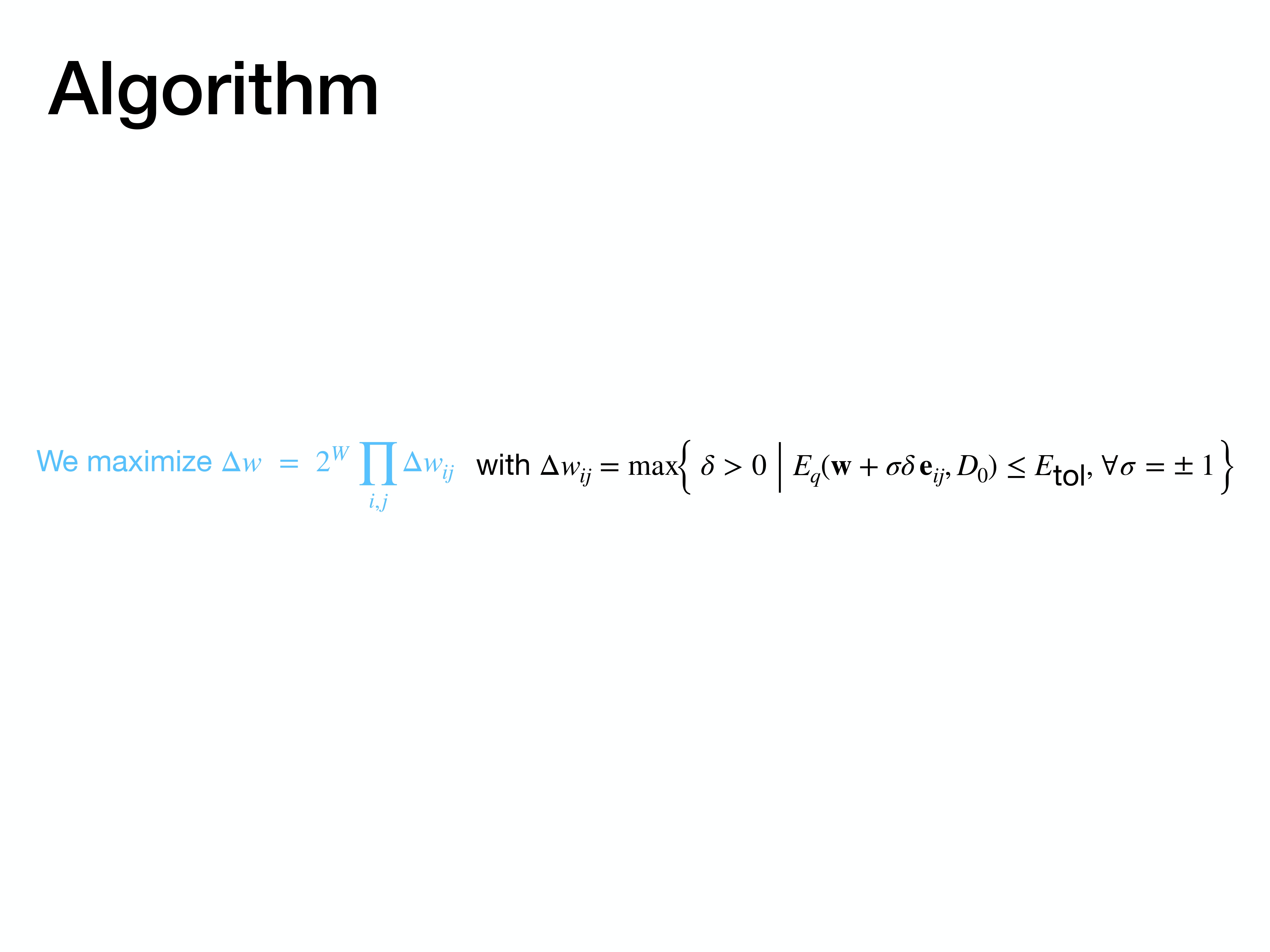
This slide reiterates the goal, explicitly showing the formula for the box volume and reminding us that each edge of the box, $\Delta w_{ij}$, is defined by how much a weight can change before the error surpasses a set tolerance.
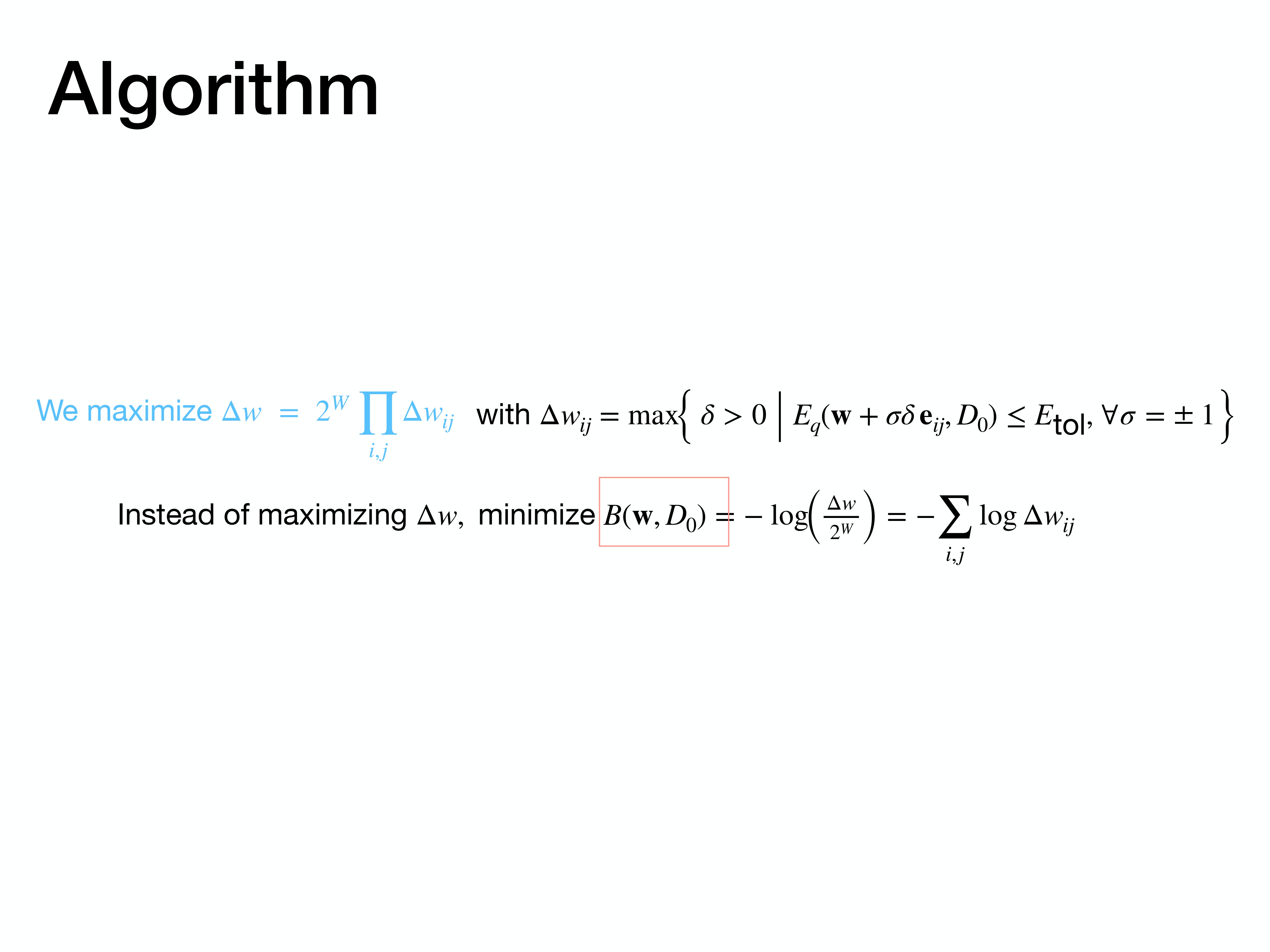
Maximizing a product of many terms is difficult. A standard trick is to instead minimize the negative logarithm of the value. Here, we shift our objective from maximizing the volume $\Delta w$ to minimizing $B(w, D_0)$, which is proportional to the negative log of that volume.
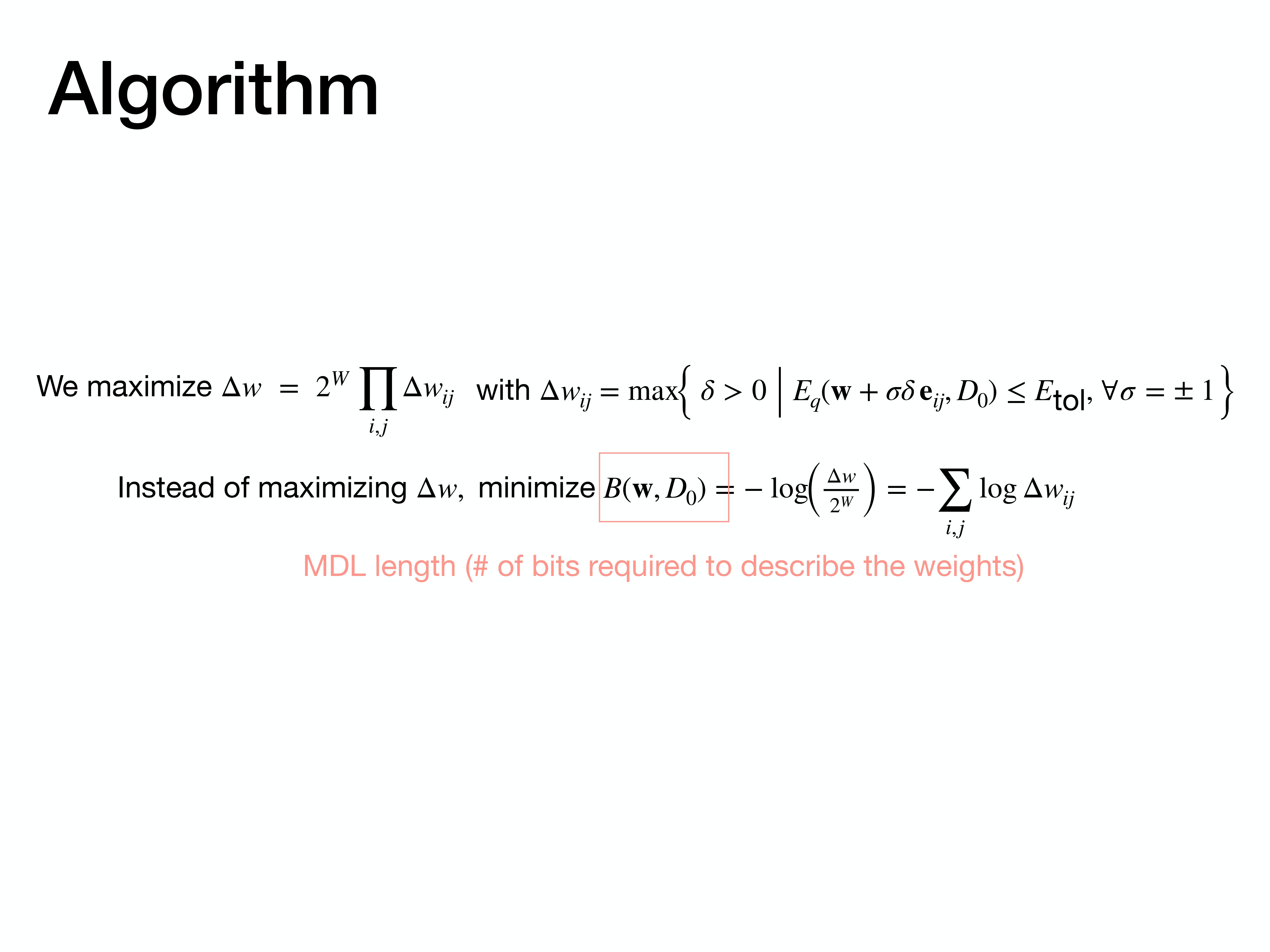
This new objective function has a nice connection to the Minimum Description Length (MDL) principle. Minimizing this term is equivalent to finding a set of weights that can be described with the fewest number of bits, which corresponds to a simpler model.
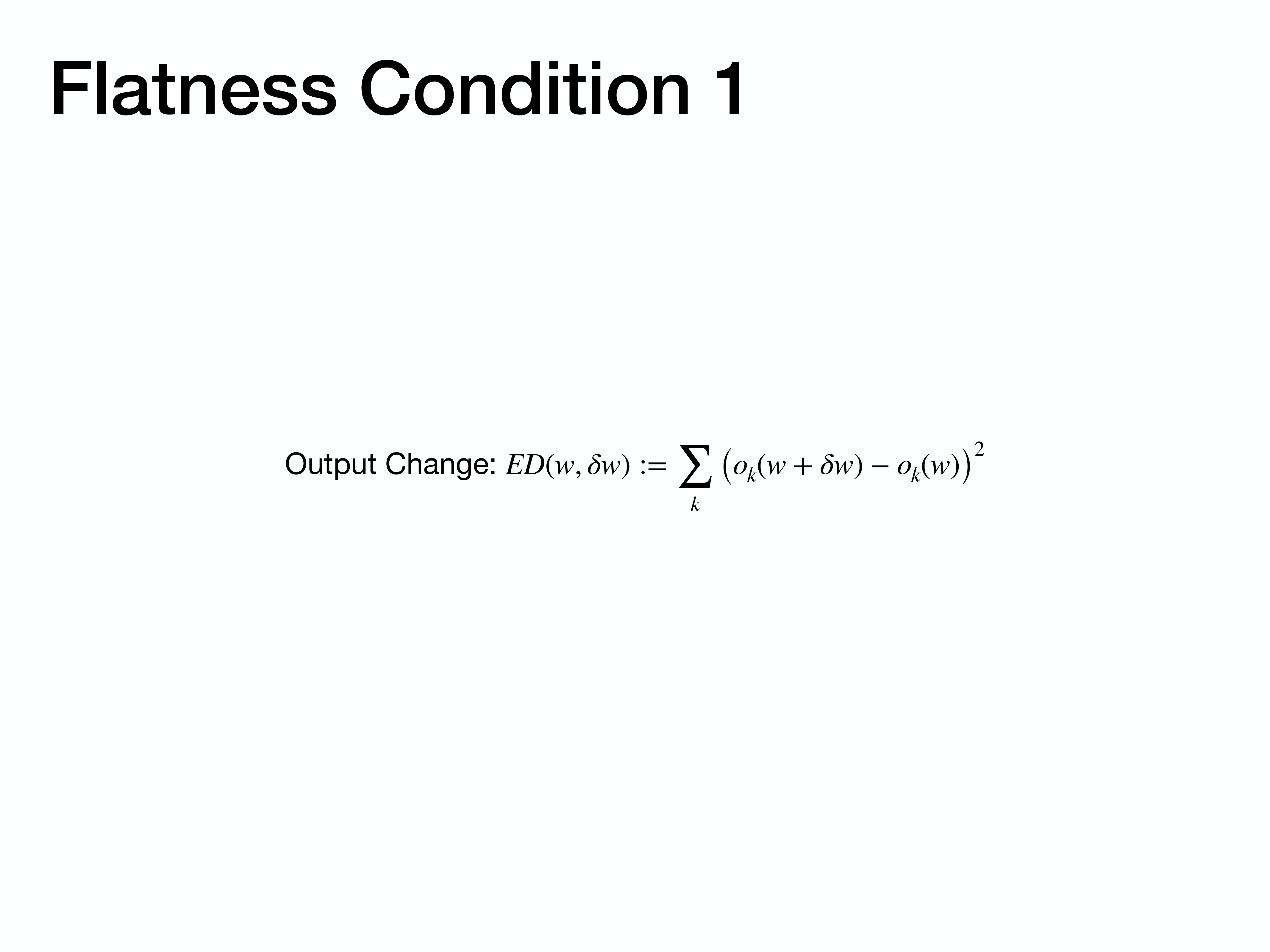
To build the algorithm, we first need to mathematically define “flatness”. We start by defining the change in the network’s output, $ED(w, \delta w)$, that results from a small change in weights, $\delta w$.
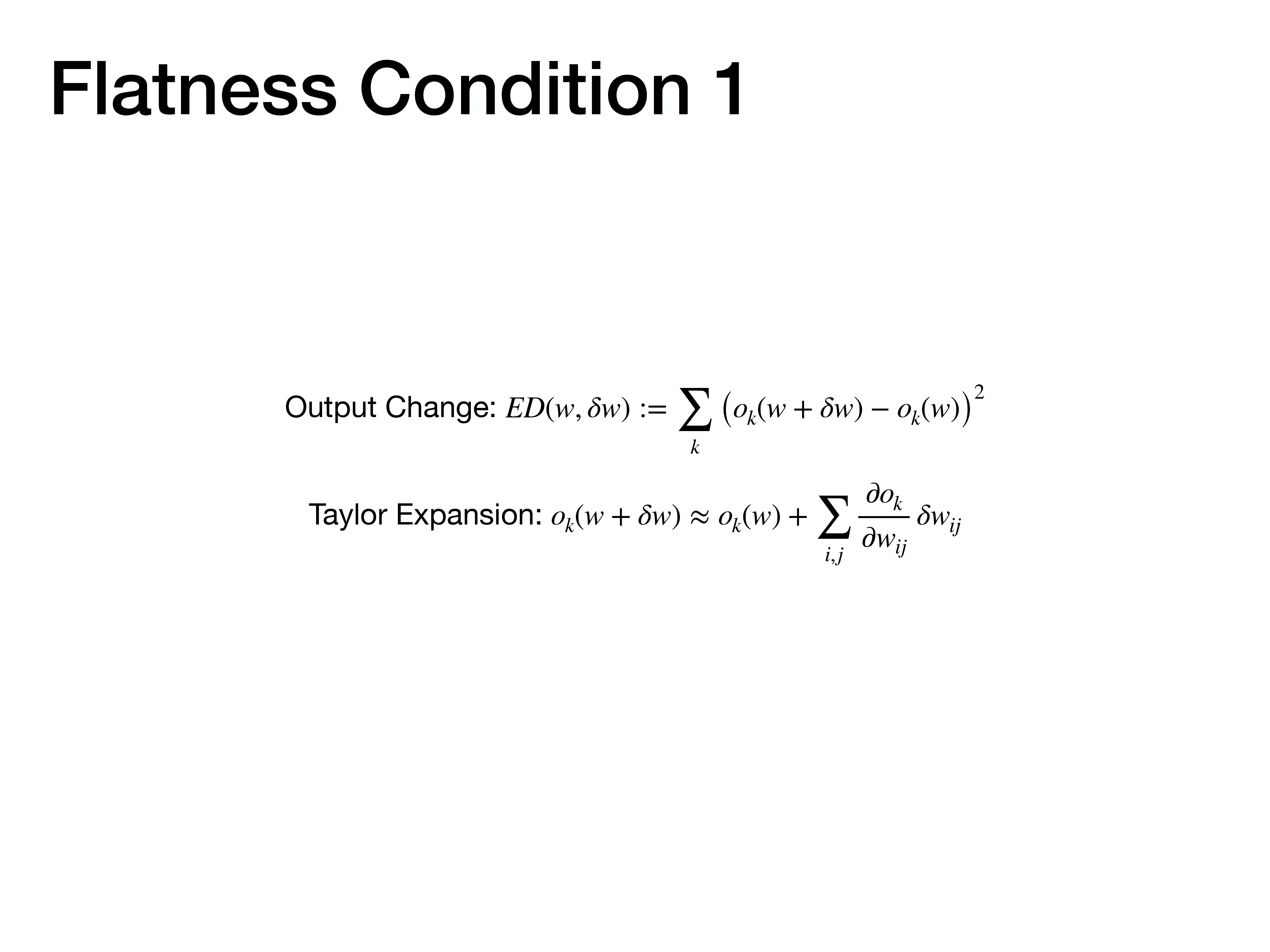
To make this expression for output change usable, we approximate it using a first-order Taylor expansion. This allows us to express the new output, $o_k(w + \delta w)$, in terms of the original output and the first derivatives (gradients).
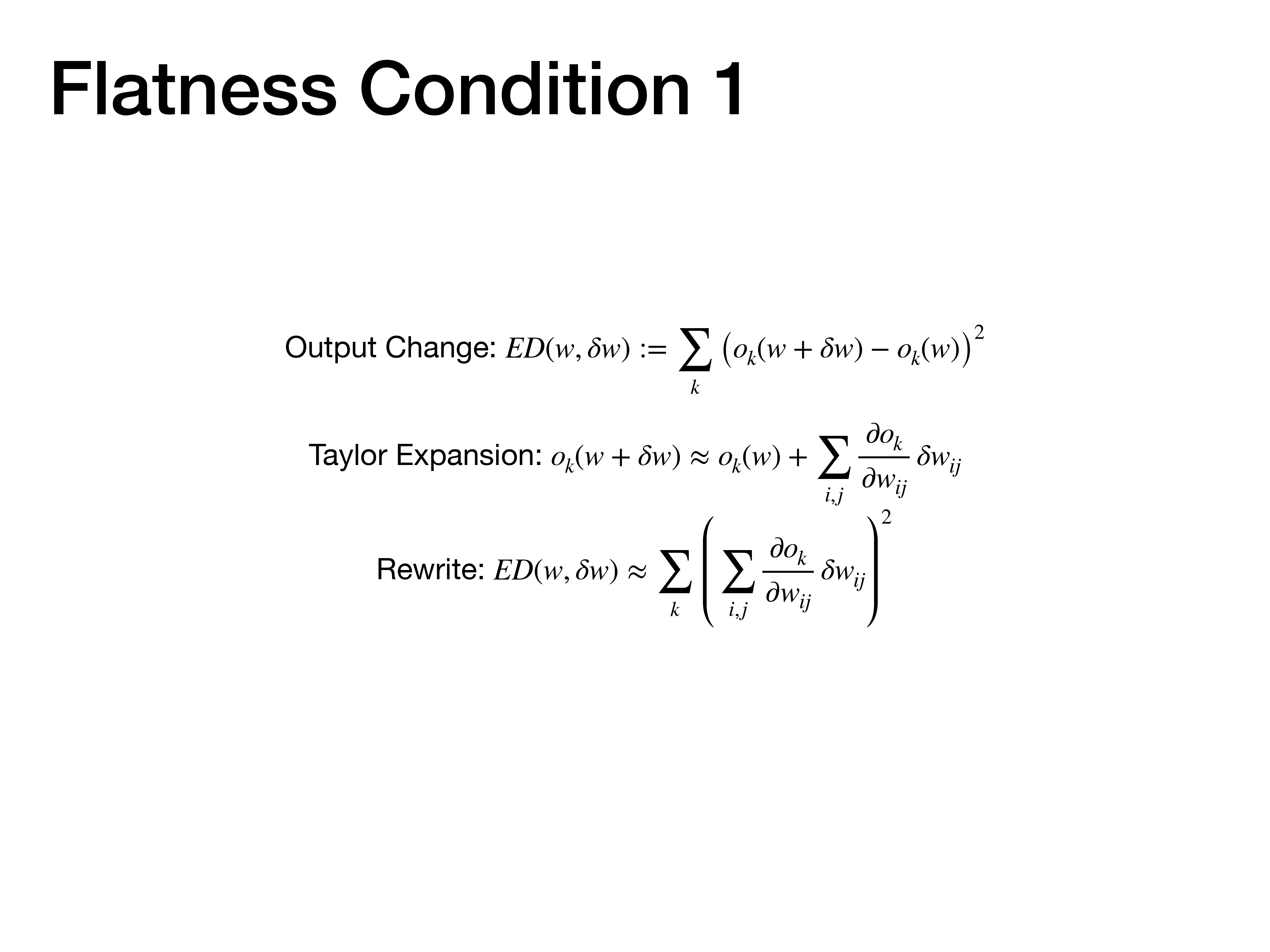
Substituting the Taylor expansion back into our definition of output change gives us an approximate formula that depends on the sum of gradients multiplied by the weight changes.
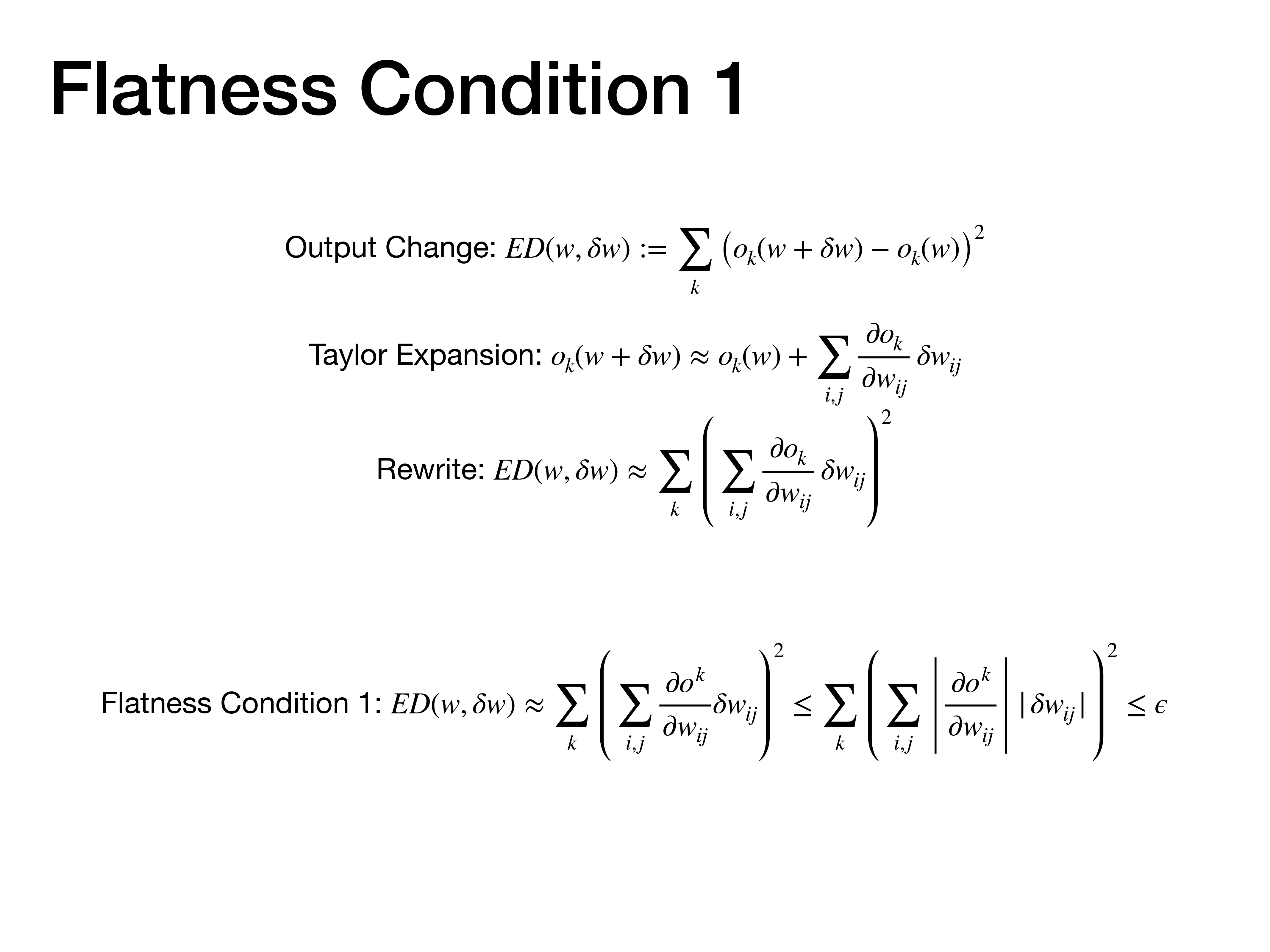
This leads to our first flatness condition: for a minimum to be considered flat, the total change in output resulting from a weight perturbation must be less than or equal to some small constant, c. This ensures that small weight changes don’t lead to large output changes.
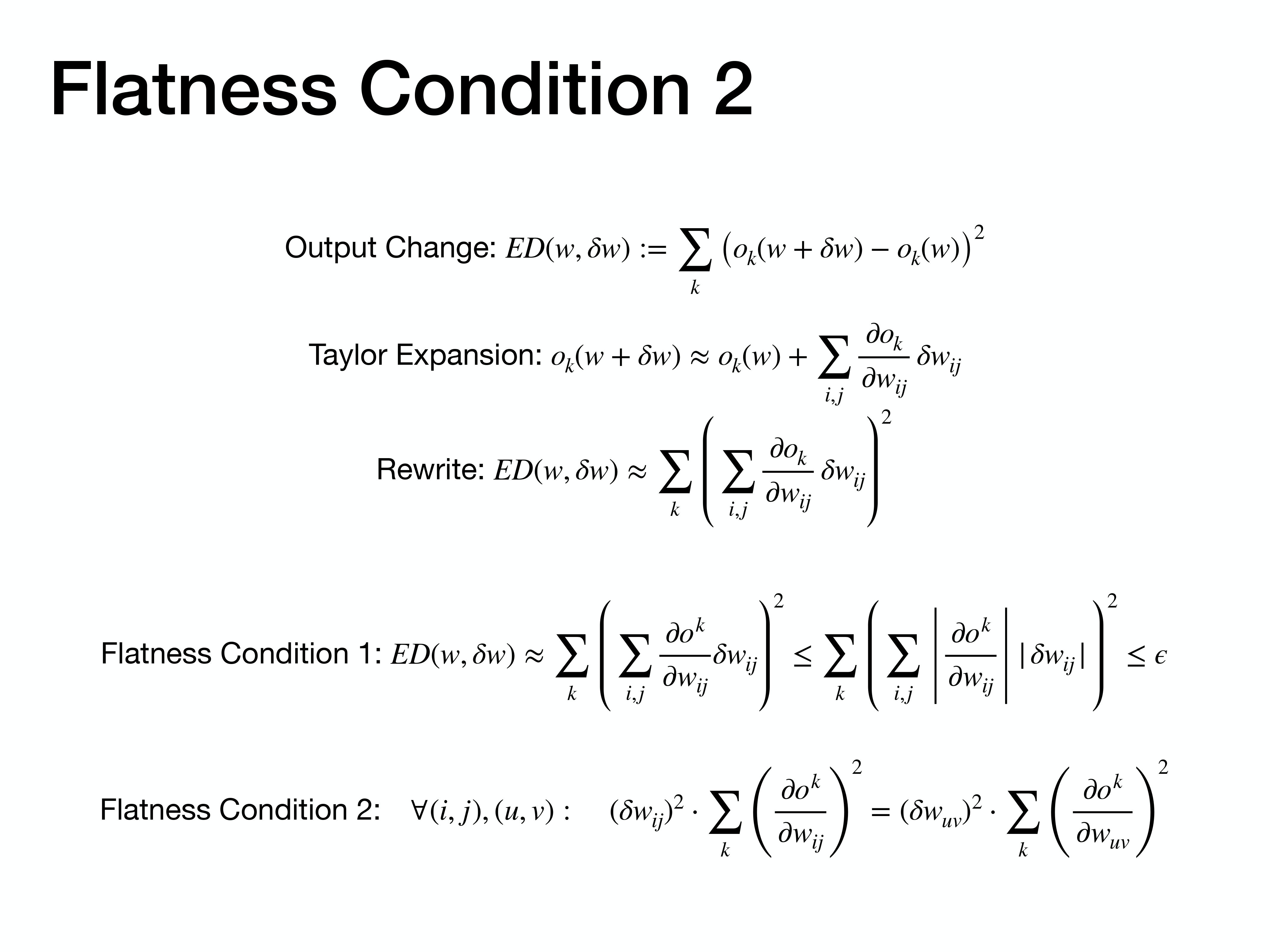
The second condition is designed to maximize the volume of our hyper-cuboid. To do this, we want to make the box as “spherical” as possible by ensuring that perturbations to each weight contribute equally to the total output change.
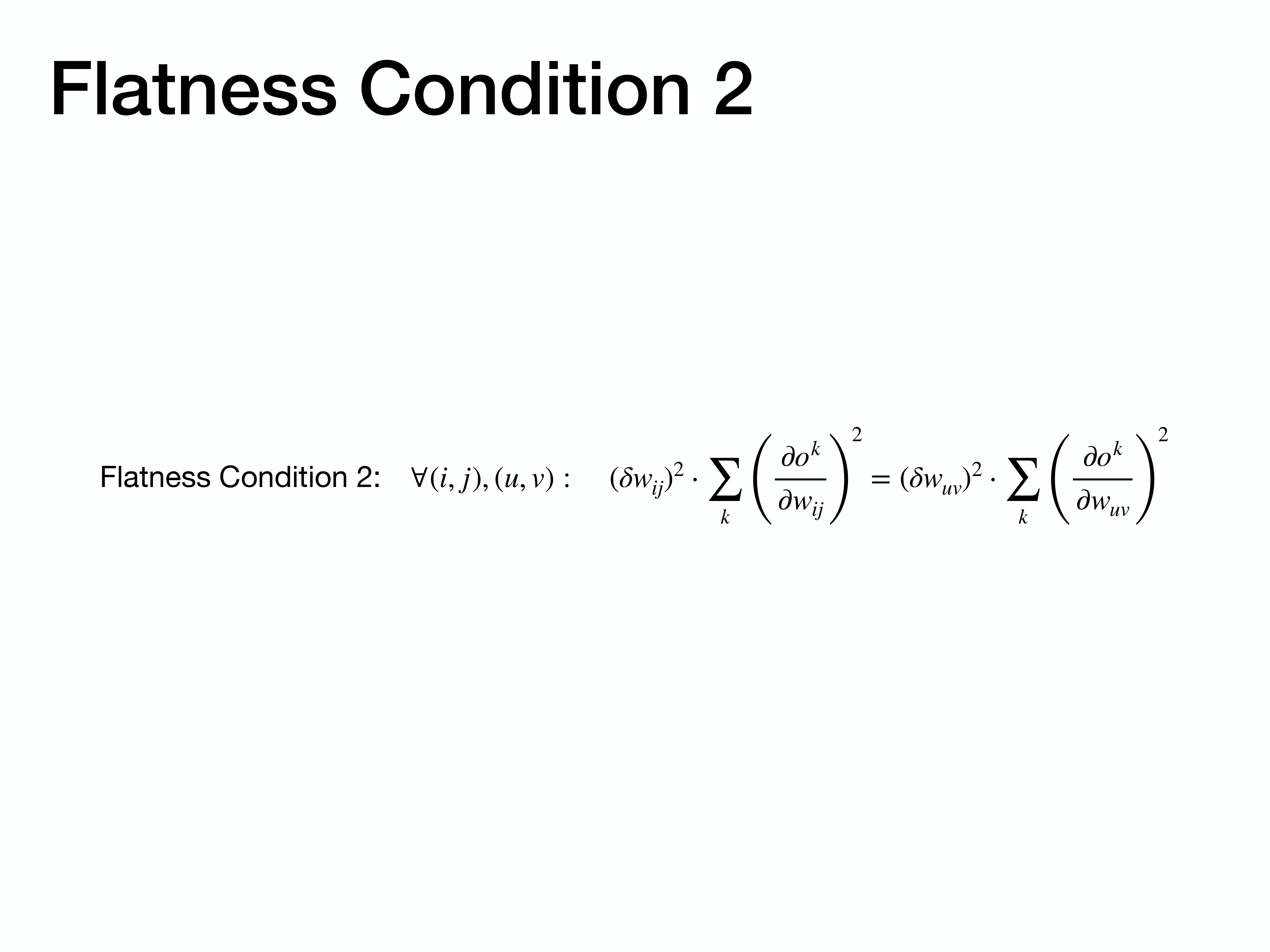
Here is a clearer statement of Flatness Condition 2. It sets an equality: the output change caused by perturbing weight $w_{ij}$ should be equal to the output change caused by perturbing any other weight $w_{uv}$.
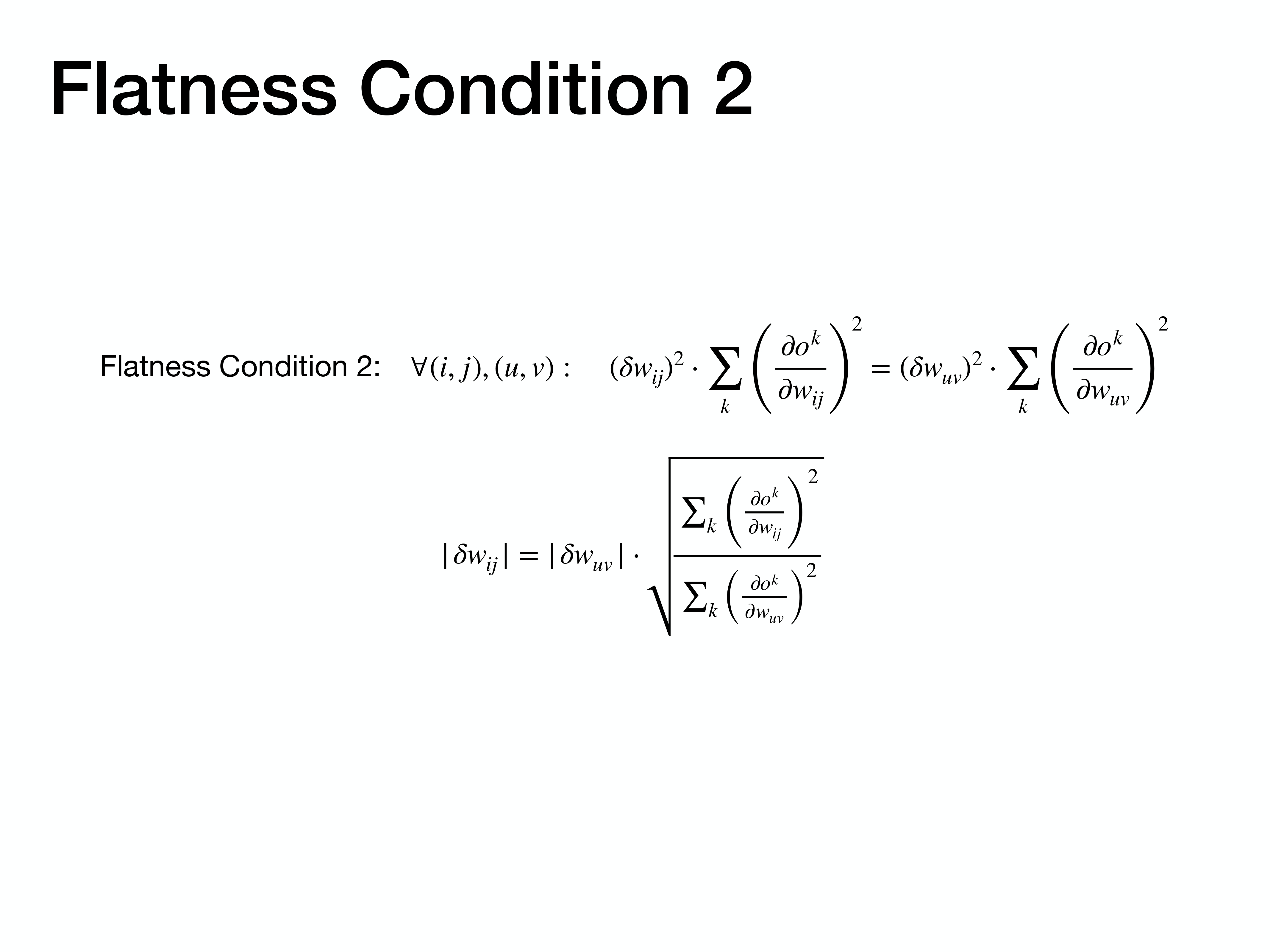
By rearranging the equation from Condition 2, we can express the allowable perturbation for one weight, $|\delta w_{ij}|$, in terms of the perturbation of another weight and the ratio of their sensitivities (measured by their output gradients).
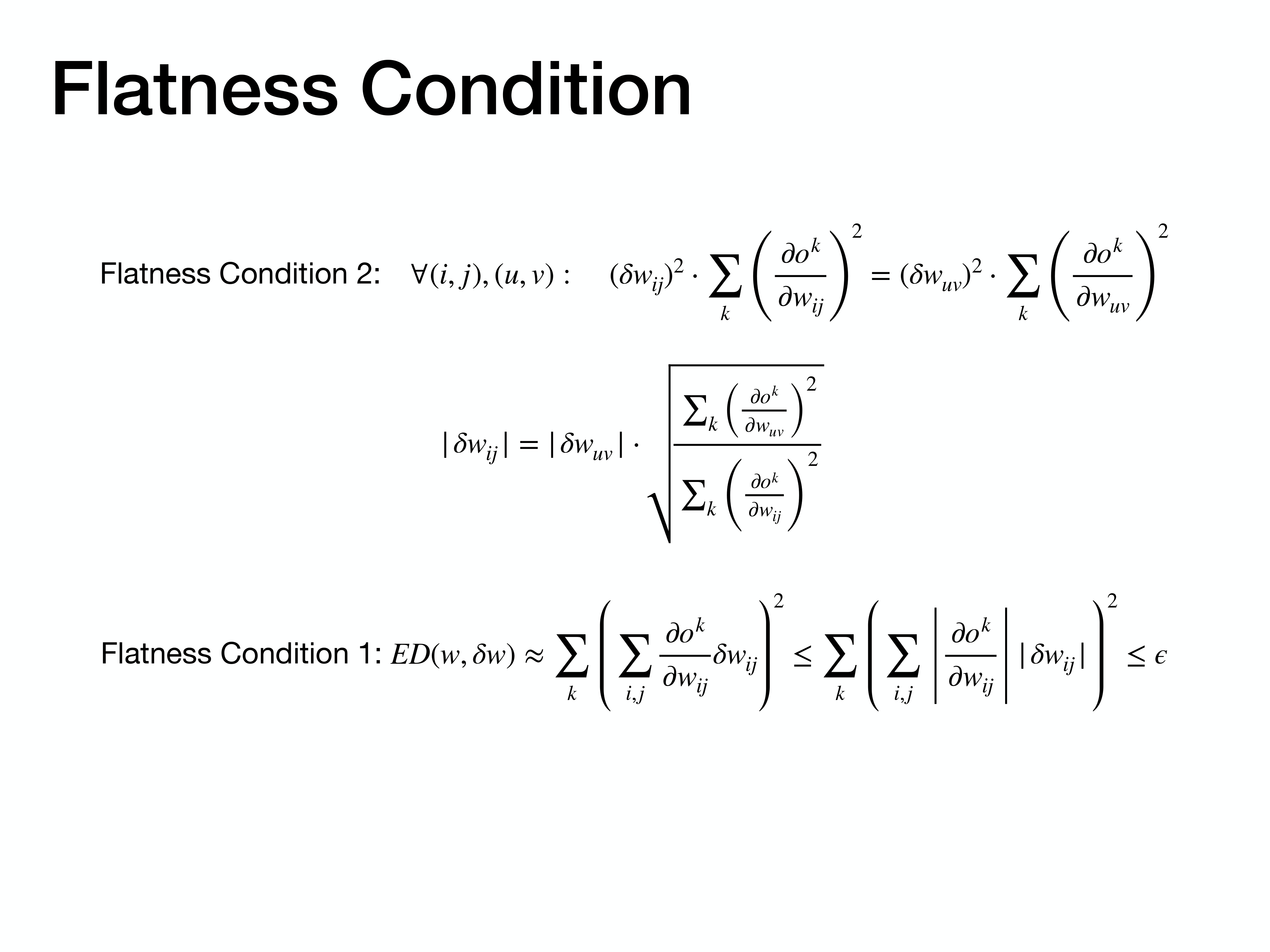
This slide simply presents both flatness conditions together, showing how they combine to define the properties of the solution we are seeking.
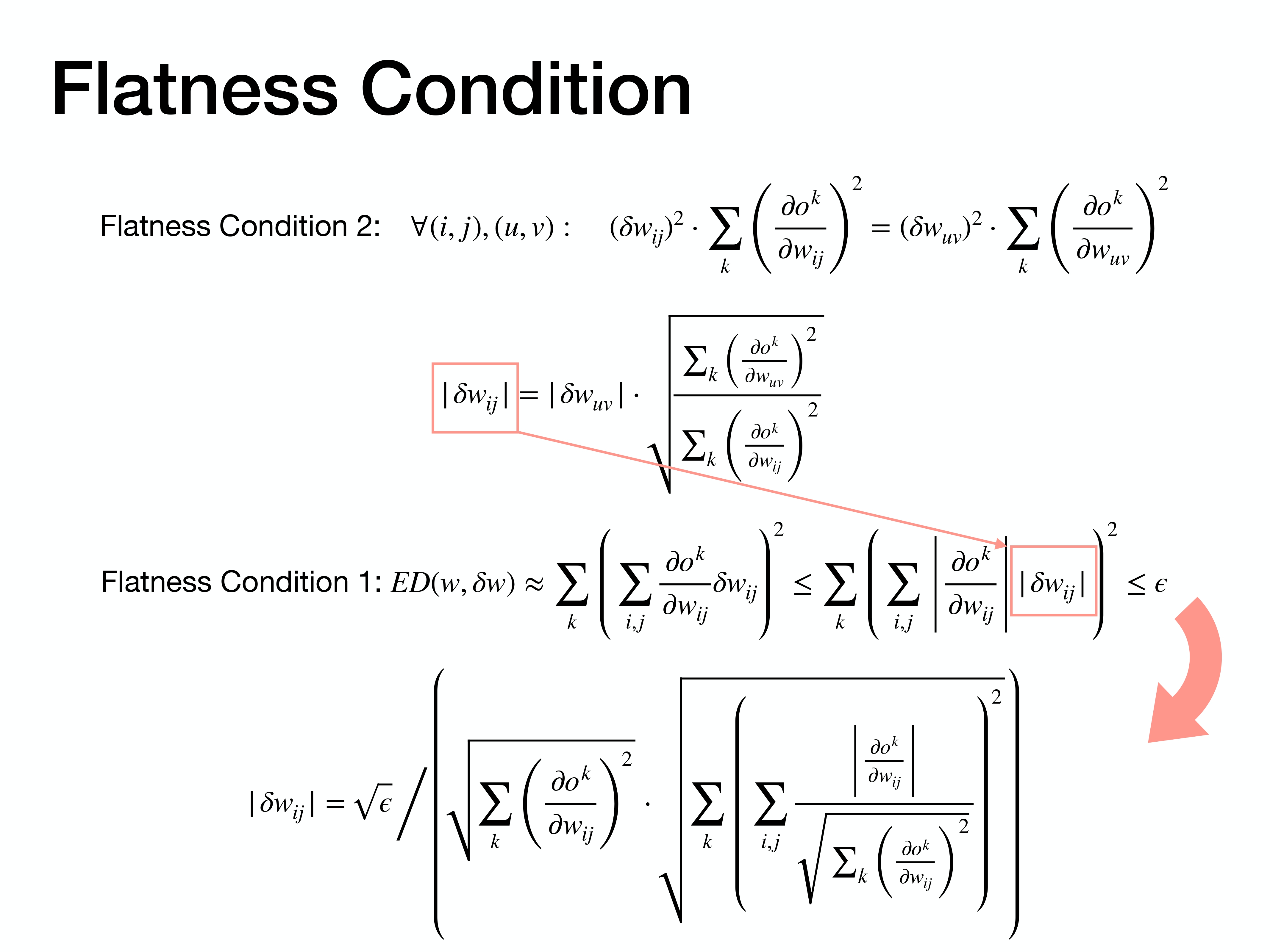
By solving the system of equations defined by both flatness conditions, we arrive at a final formula for the maximum allowable perturbation for any given weight, $|\Delta w_{ij}|$. This formula depends on the network’s output gradients.
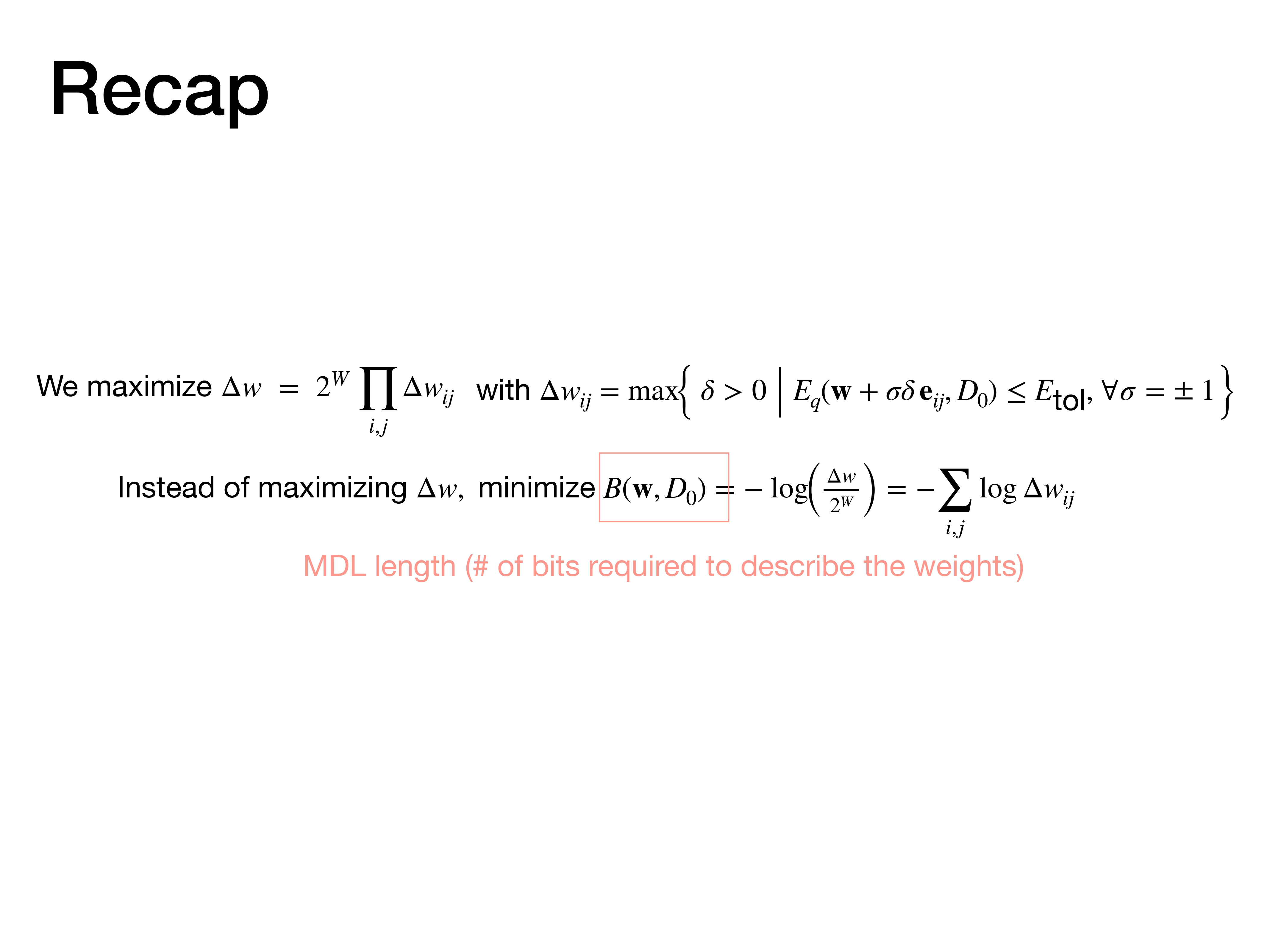
Let’s quickly recap the algorithm’s goal. We aim to maximize the box volume $\Delta w$, which is equivalent to minimizing the MDL cost function $B(w, D_0)$.
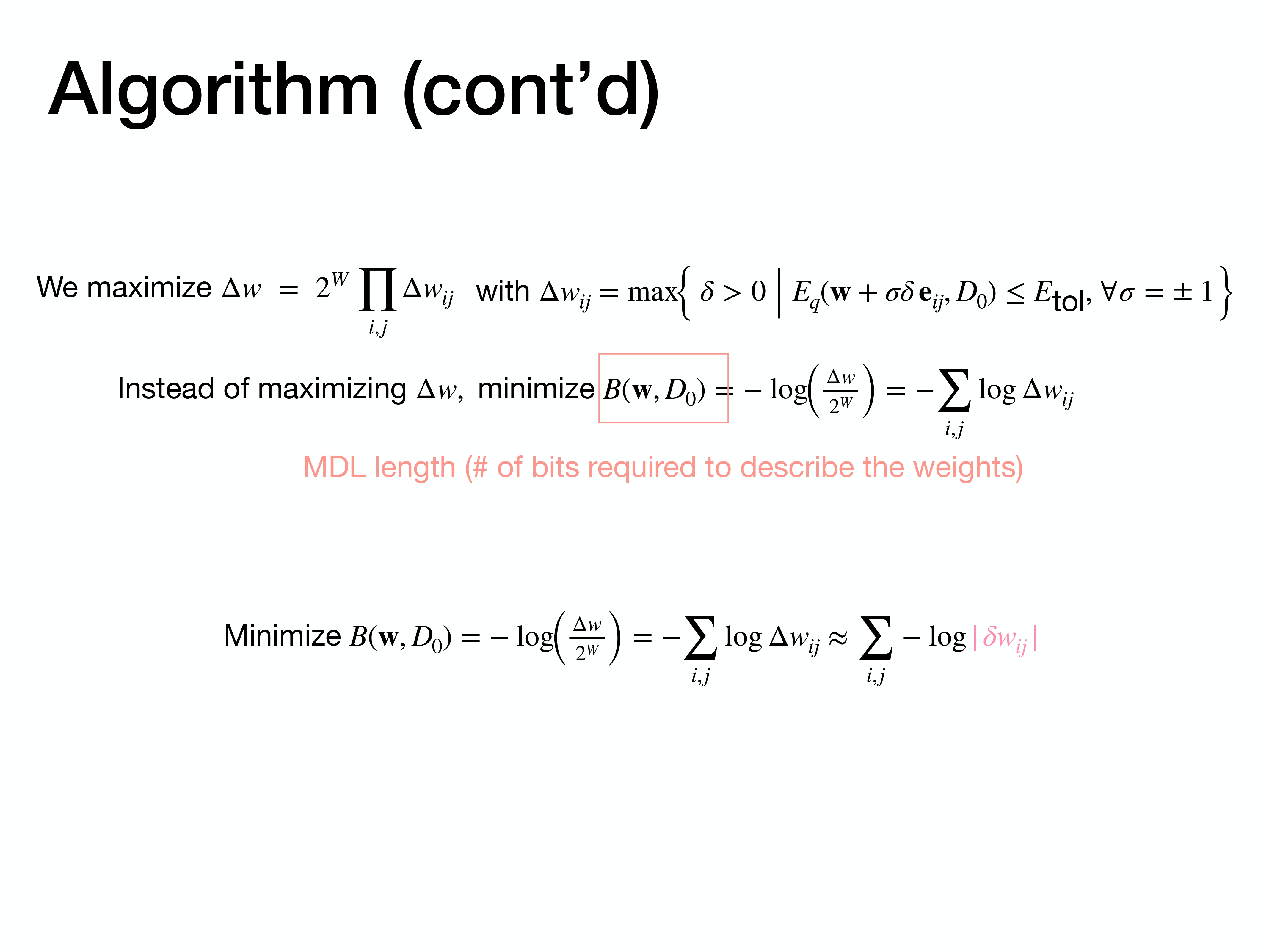
Now that we have a formula for the size of the box edges, $\Delta w_{ij}$, we can express our cost function $B(w, D_0)$ in terms of the network’s derivatives. This slide shows that connection, approximating the log of $\Delta w_{ij}$ with the log of the derived formula.
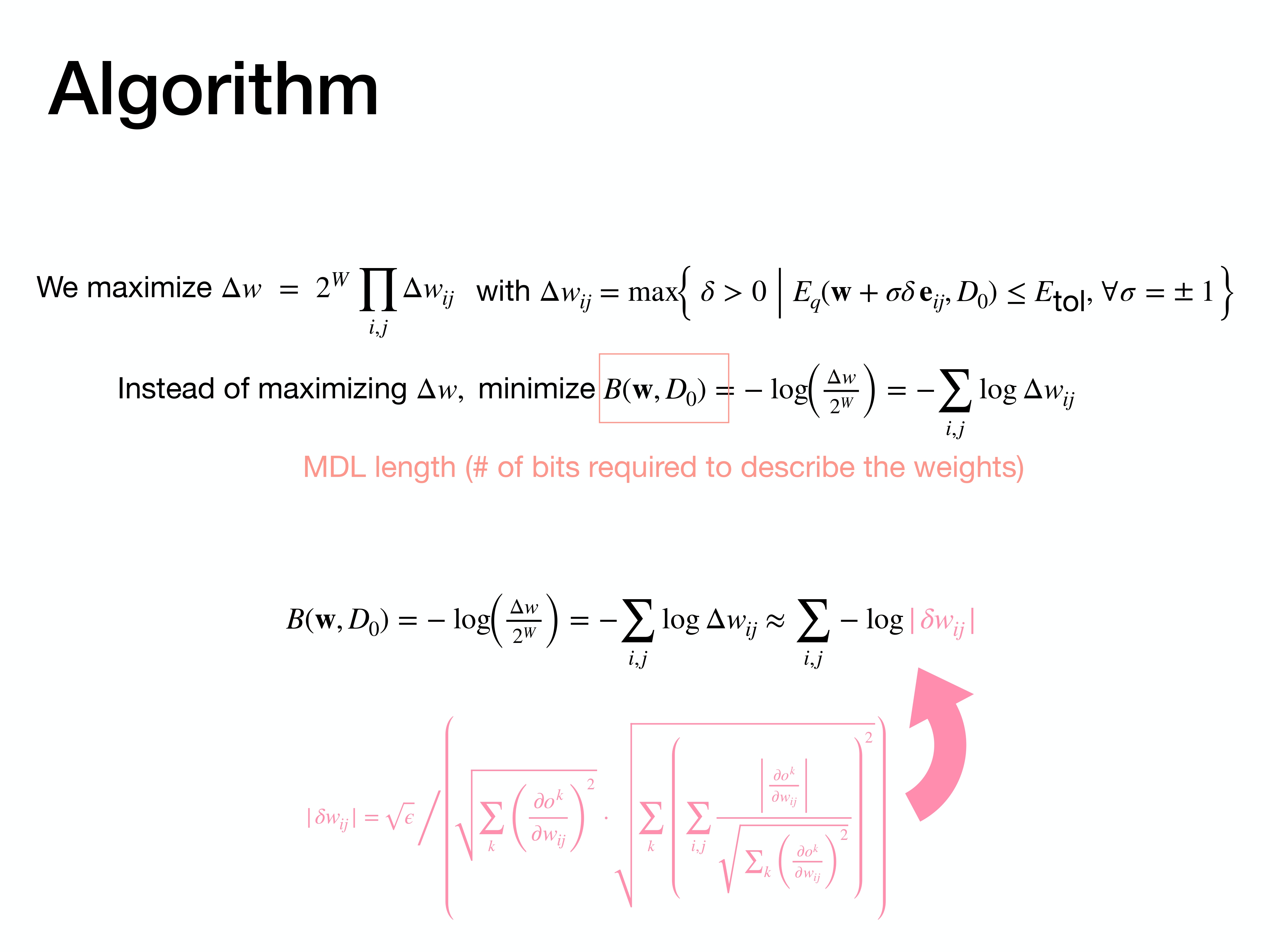
This slide restates the formula for the size of the perturbation $|\Delta w_{ij}|$, which is the key result from our derivation using the two flatness conditions.
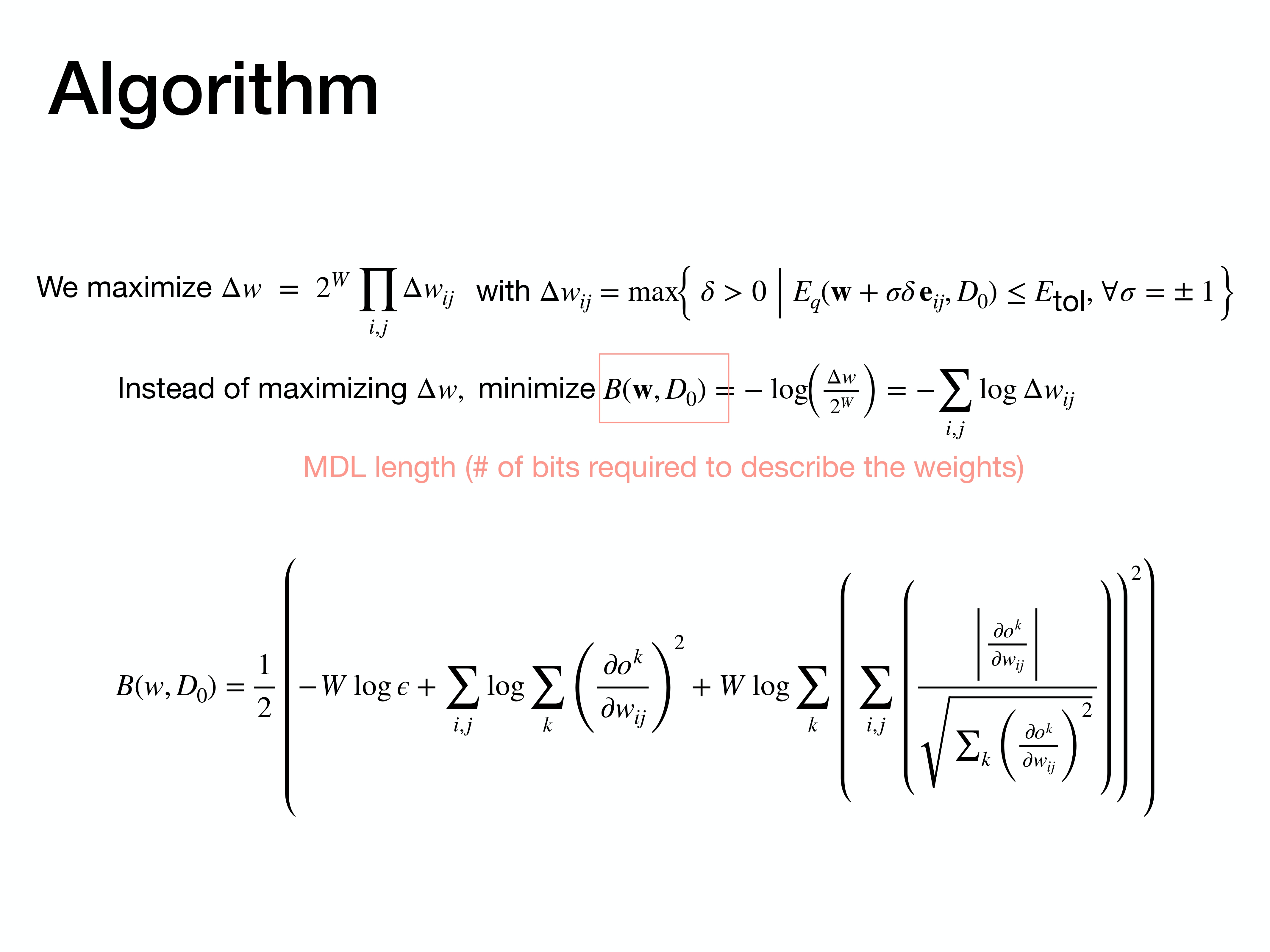
Plugging the expression for $\Delta w_{ij}$ into our cost function $B(w, D_0) = -\sum \log \Delta w_{ij}$ gives us this final, albeit complex-looking, penalty term that we need to minimize. This term explicitly captures the “flatness” of the minimum.
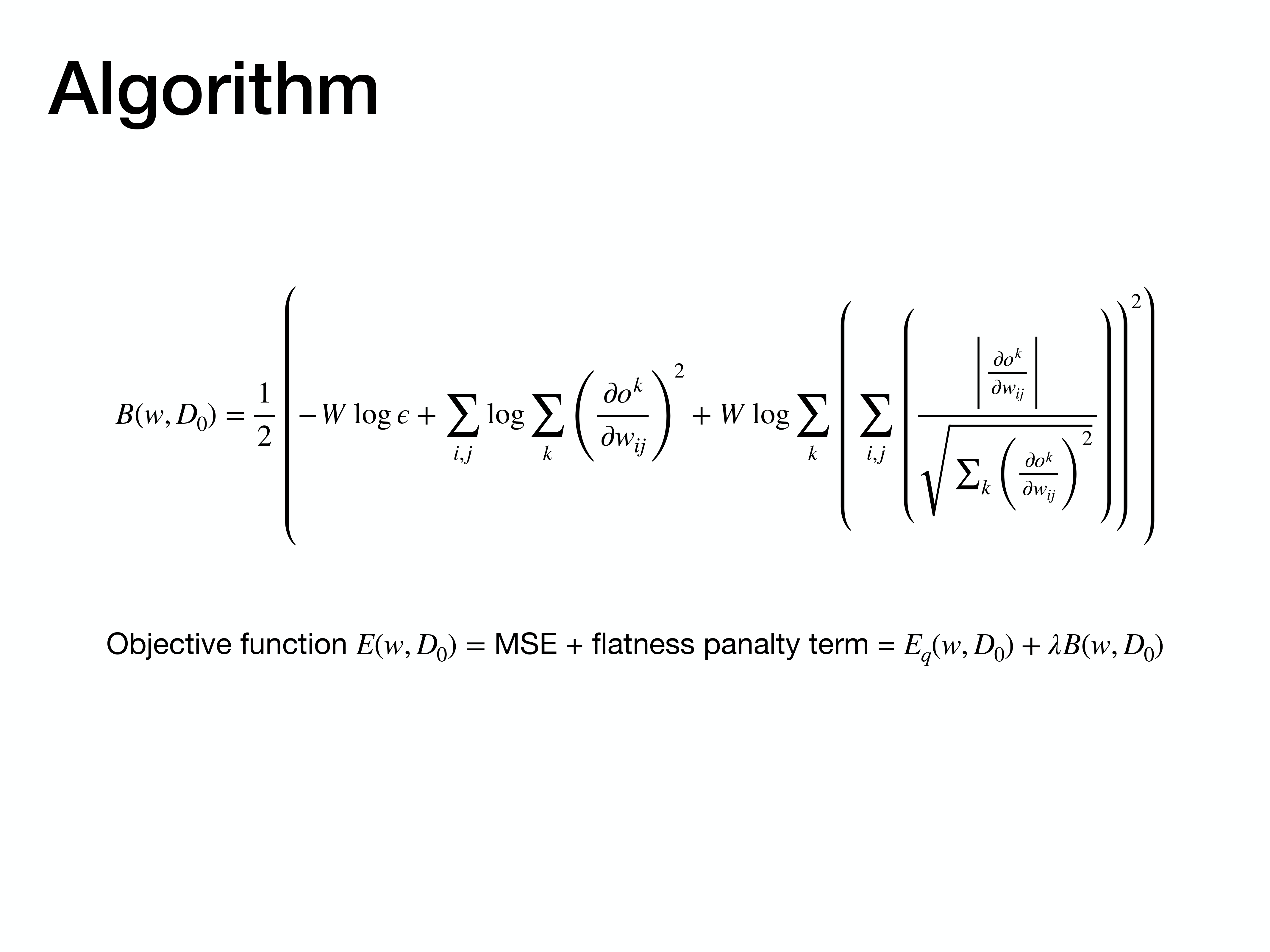
The complete objective function for training is then a combination of two parts: the standard MSE, which ensures the model fits the training data, and our new flatness penalty term, which encourages the model to find a simple, generalizable solution. A hyperparameter $\lambda$ balances the two.
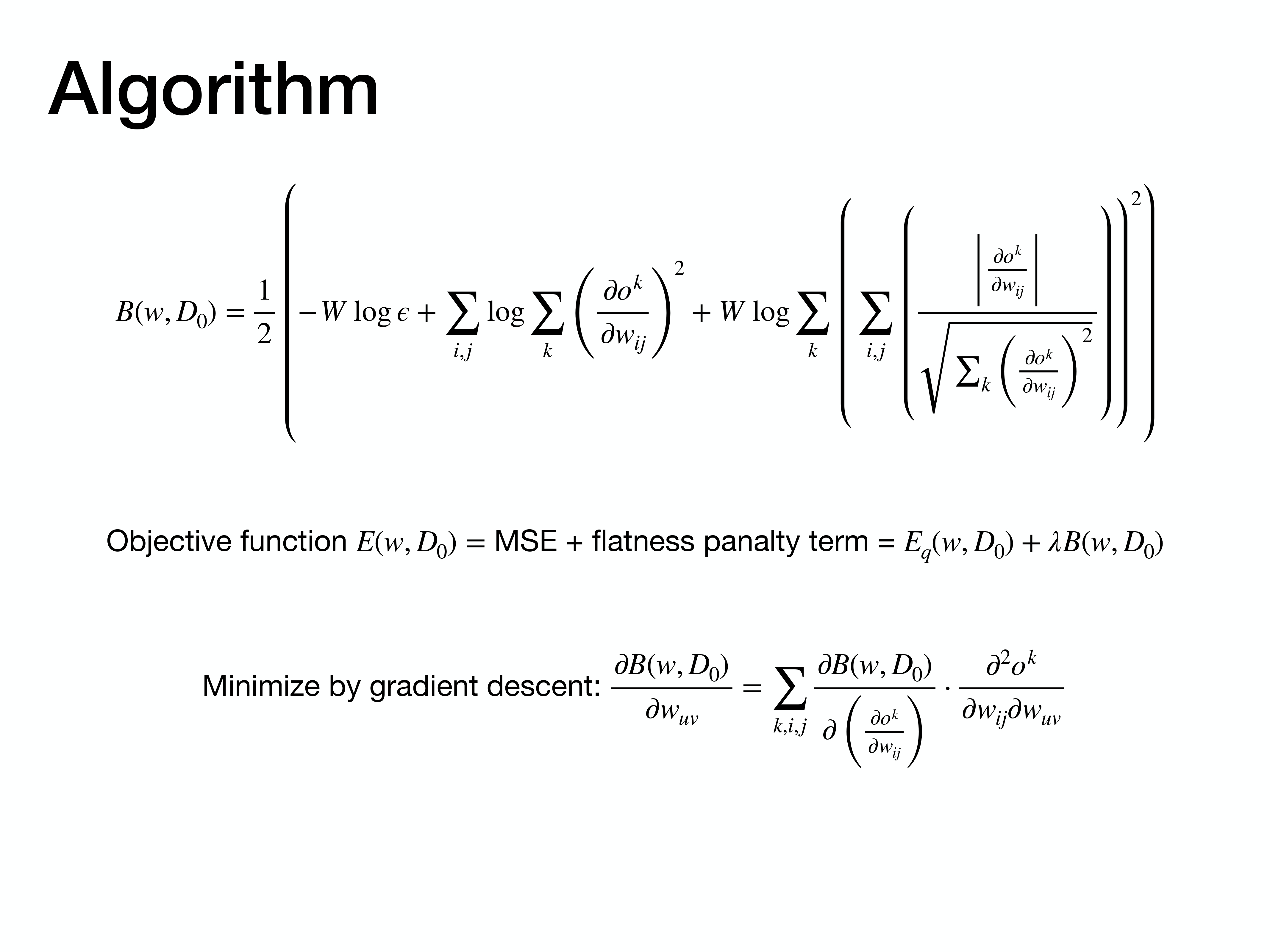
To minimize this objective function using gradient descent, we need to compute its gradient. The gradient of the flatness penalty term involves second-order derivatives of the network’s output, which would typically be very expensive to compute.
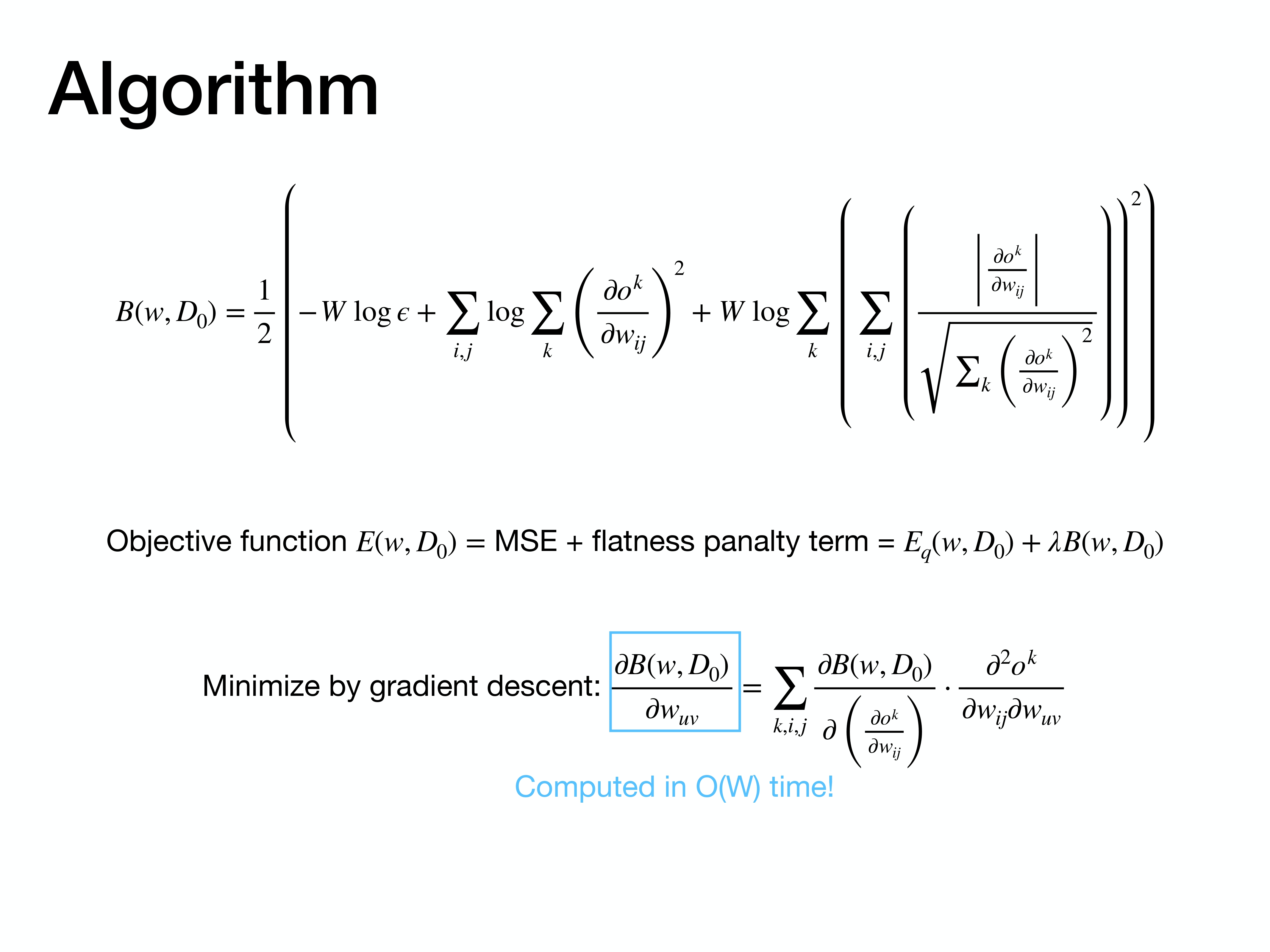
However, the paper leverages a crucial insight. This complex gradient, which involves second-order information, can be calculated with a computational complexity of $O(W)$—the same as standard backpropagation—using a technique known as the Pearlmutter trick. This makes the entire algorithm practical and efficient.
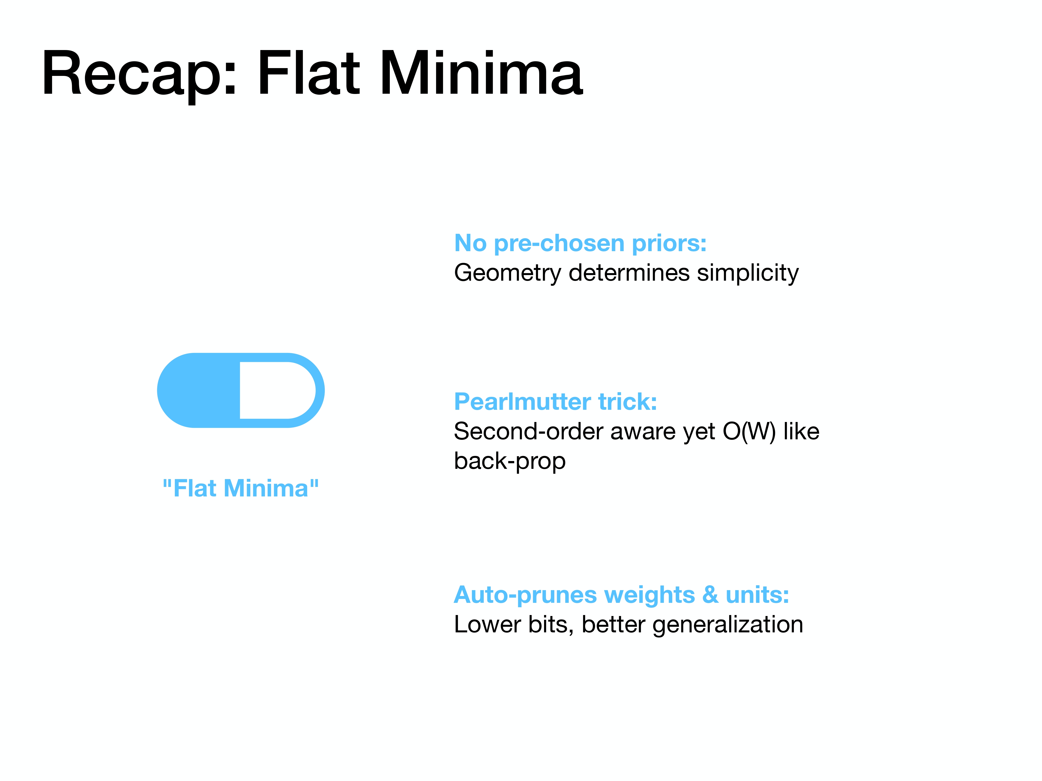
To recap the key advantages: the “Flat Minima” method is appealing because it uses geometry instead of priors to define simplicity, it’s computationally efficient, and it naturally performs network pruning for better generalization.
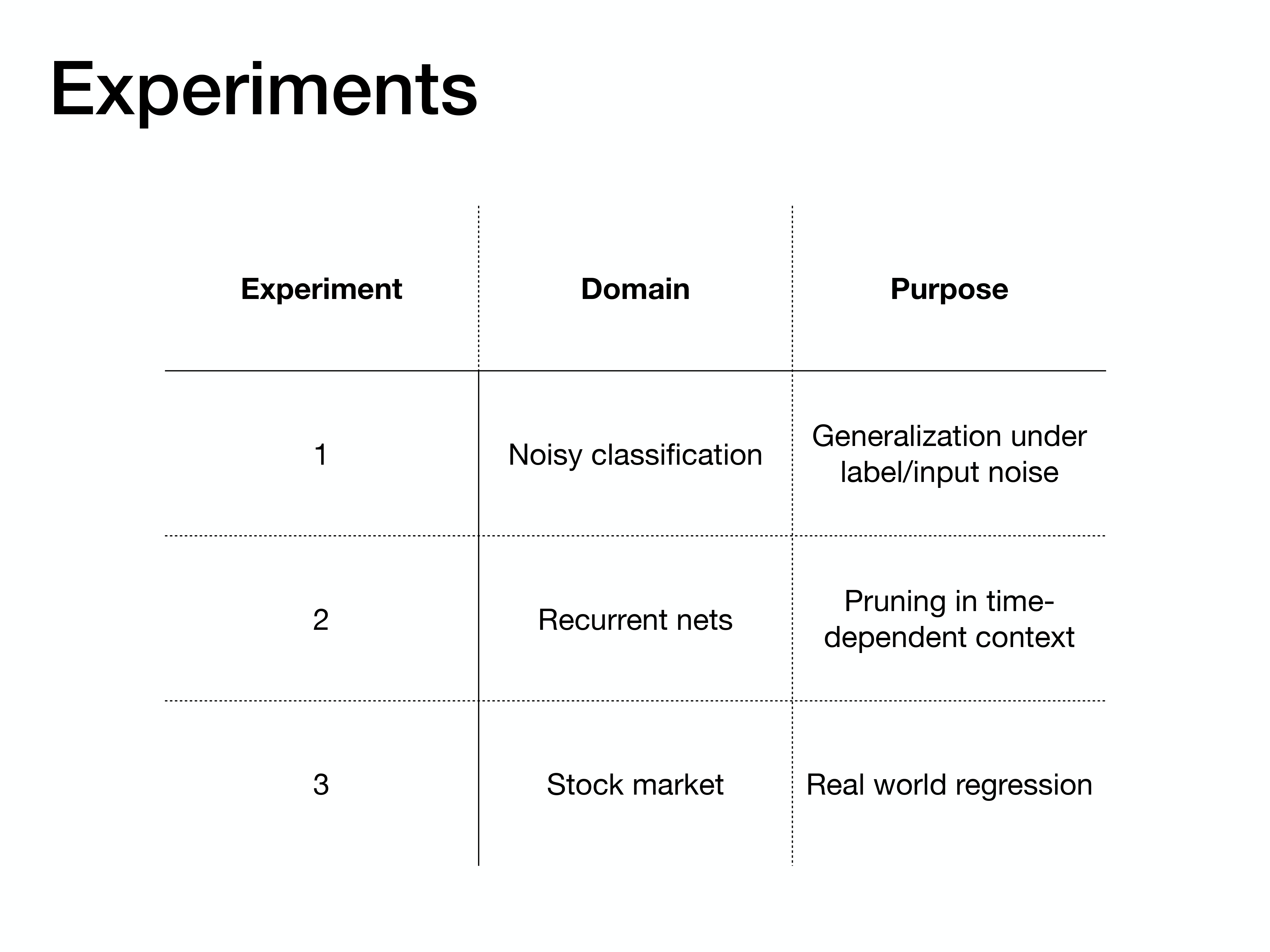
The paper then presents three experiments to prove the effectiveness of the algorithm. These tests cover noisy classification, a recurrent network task, and a real-world regression problem using stock market data.
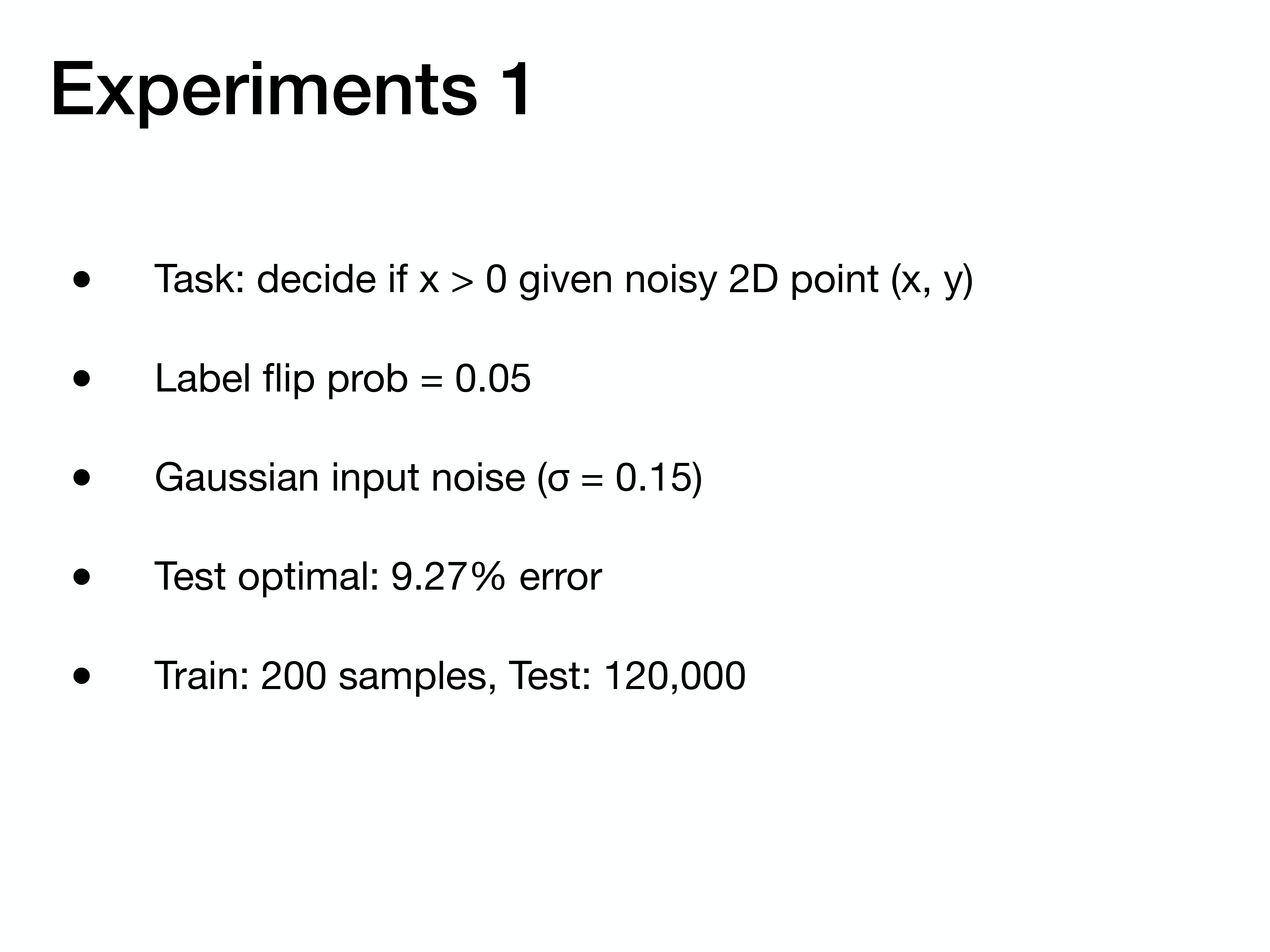
In the first experiment, the task was to classify a 2D point with both label and input noise. The network was trained on a small set of 200 samples and tested on a very large set of 120,000 samples to reliably measure generalization.
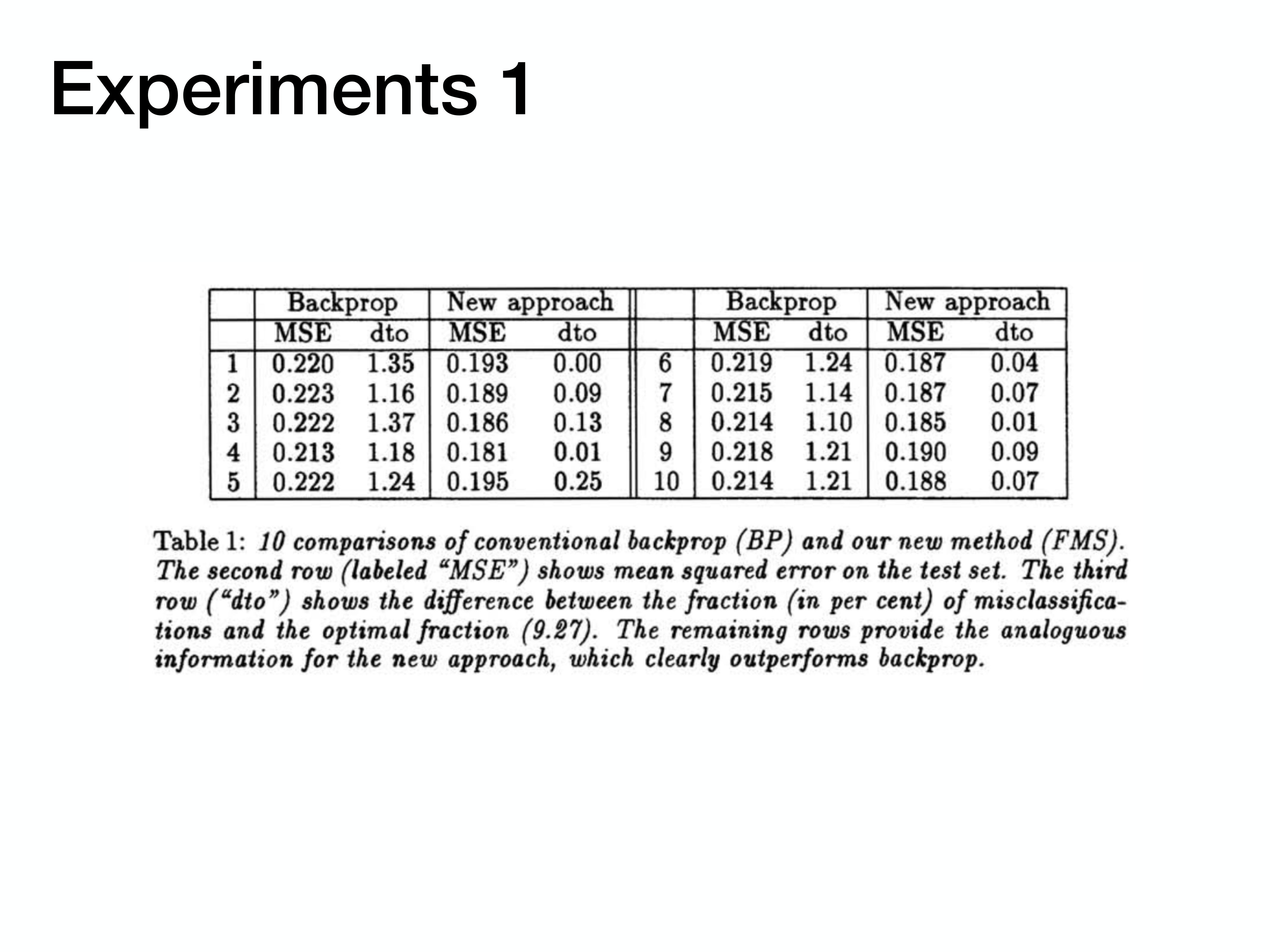
The results of the first experiment are shown here. This table presents 10 direct comparisons between conventional backprop and the new FMS approach. In every single run, the new method achieves a lower test error and gets significantly closer to the optimal error rate, clearly demonstrating superior generalization.
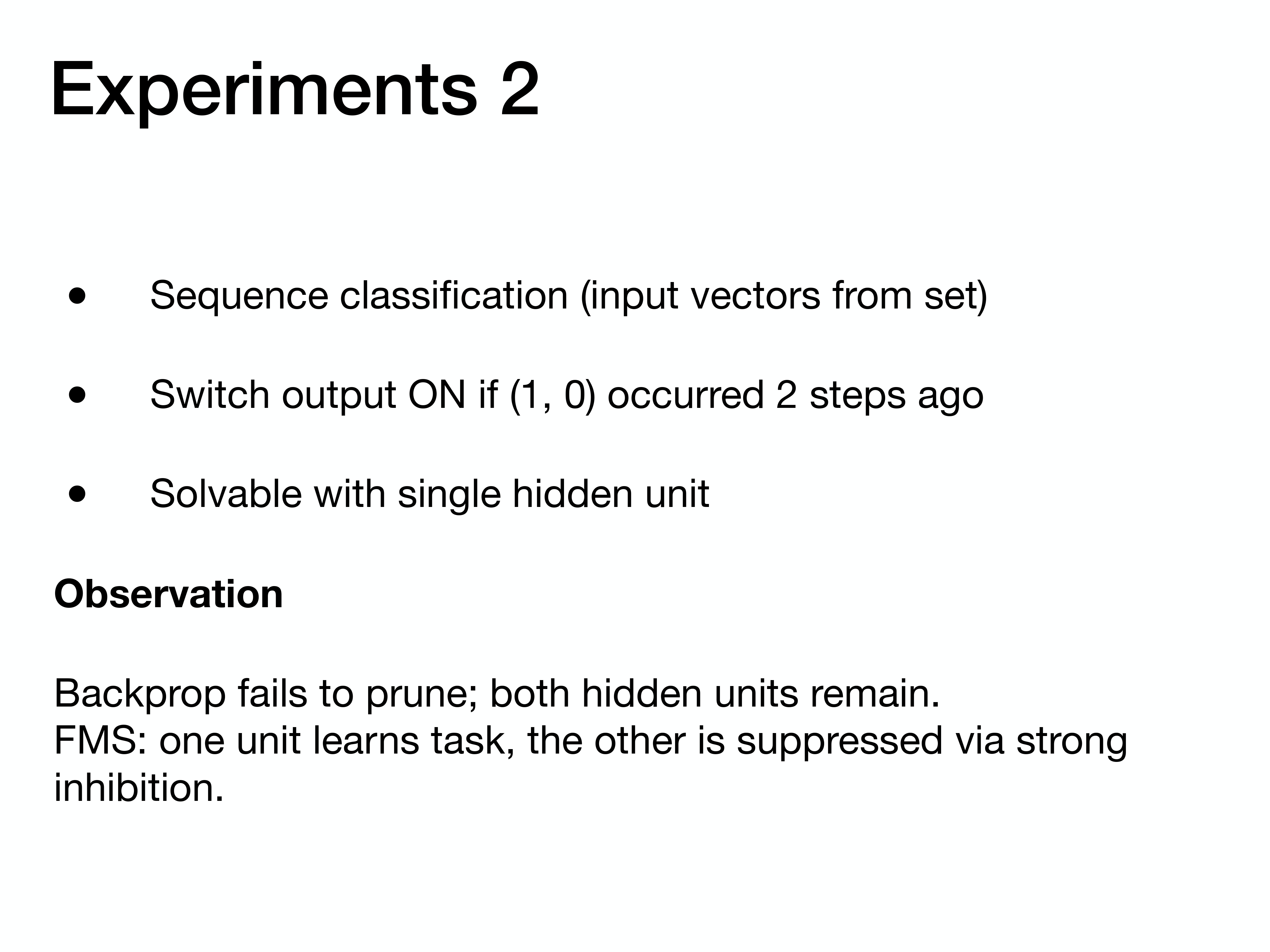
The second experiment used a recurrent neural network for a sequence classification task. The problem was designed to be solvable with just one hidden unit. While backprop failed to prune the redundant second unit, the FMS method successfully suppressed it, demonstrating its automatic model simplification capability.
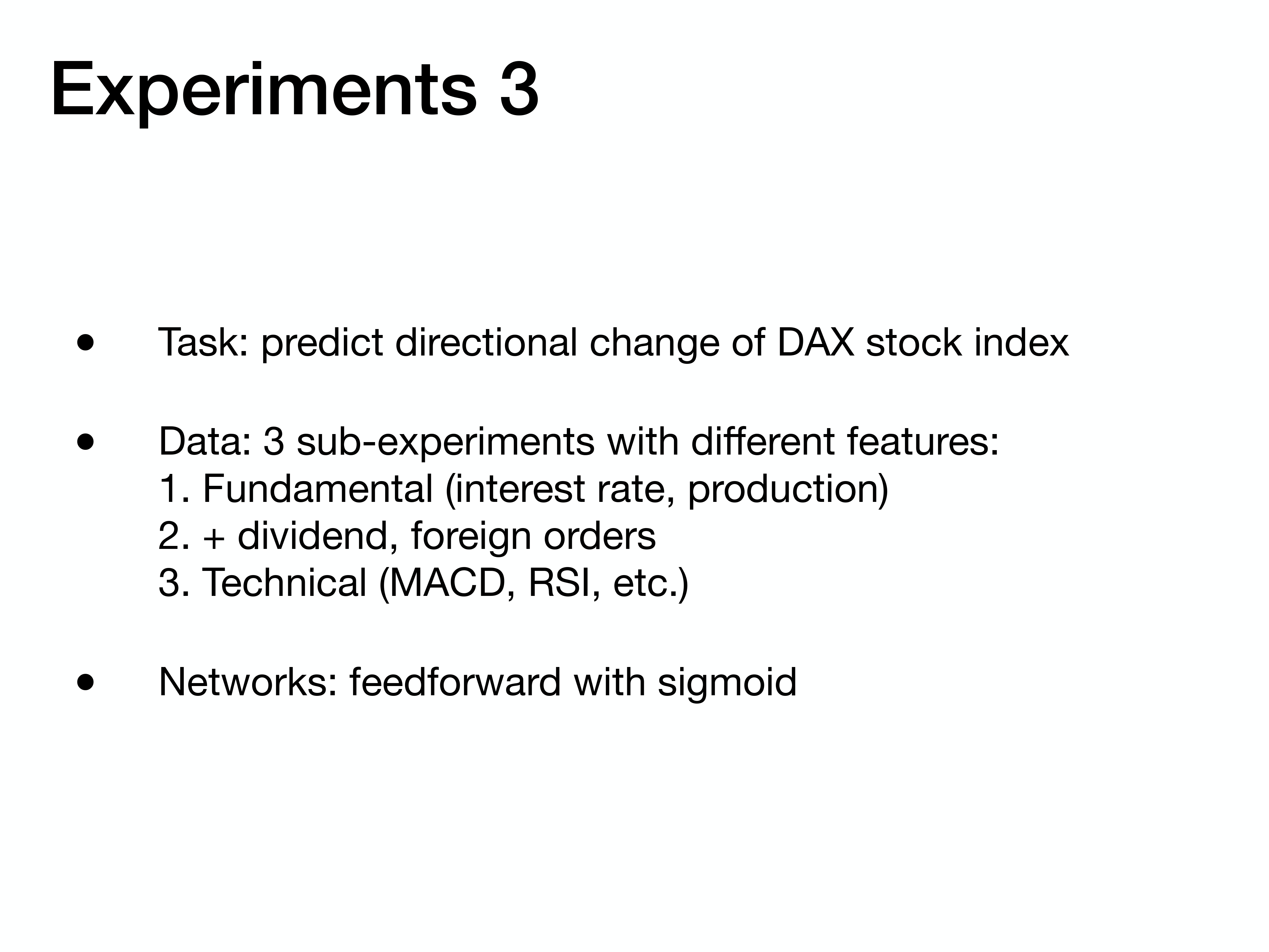
The final experiment tackled a real-world problem: predicting directional changes in the DAX stock index. They used several sets of features, from fundamental economic indicators to technical trading signals.
The results from the stock market prediction task were compelling. The FMS method was benchmarked against standard Backprop, Optimal Brain Surgeon (OBS), and Weight Decay. FMS was better across all metrics and feature sets, achieving up to a 63% relative improvement over the best competitor, proving its value on noisy, real-world data.