Diffusion Model and Its Applications

Slide 1: Diffusion Model and Its Applications

Title: Diffusion Model and its applications
Presenter: Jungmook Kang
Event: StatLet Seminar
Date: 9/4/2026

Slide 2: Reference & Resources

MIT EECS 6.S183, 6.S184
Ho et al. (2020), Denoising Diffusion Probabilistic Models
Song et al. (2021), Denoising Diffusion Implicit Models
Material: mookjsi.github.io/posts/diffusion2

Slide 3: 1. Introduction

Section 1 introduces the basic generative modeling perspective behind diffusion models.

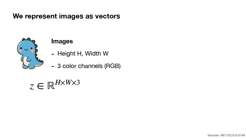
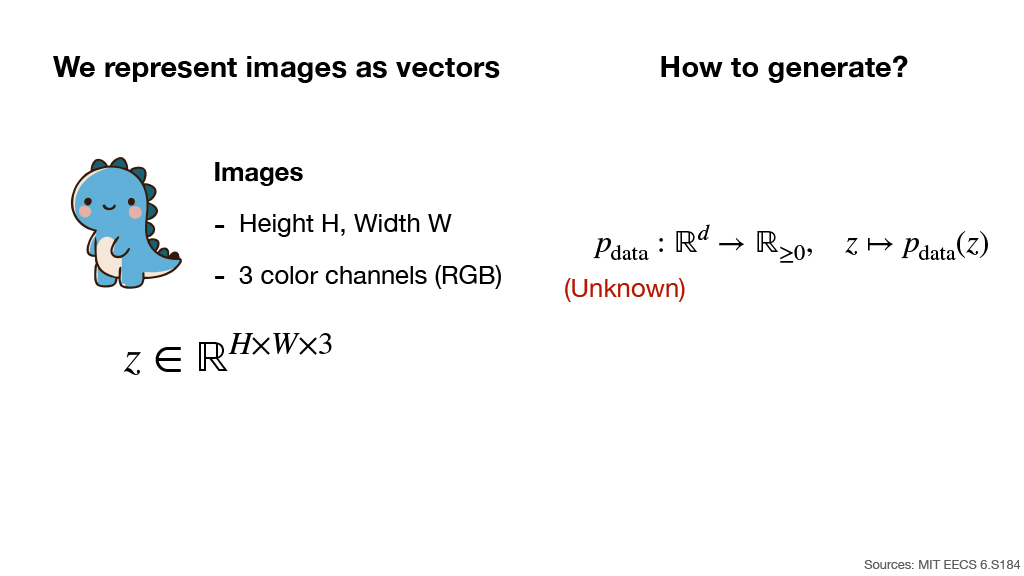
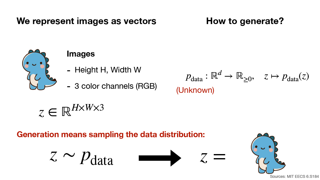
Slide 4-6: Representing Images and the Goal of Generation

Images can be represented as high-dimensional vectors.

Height: $H$
Width: $W$
Color channels: 3 channels (RGB)

$$ z \in \mathbb{R}^{H\times W\times 3} $$

Suppose the true data distribution is

$$ p_{\text{data}}:\mathbb{R}^d\rightarrow\mathbb{R}_{\ge 0}, \qquad z\mapsto p_{\text{data}}(z). $$

However, $p_{\text{data}}$ itself is unknown.

The goal of generation is to sample an image from this unknown data distribution:

$$ z\sim p_{\text{data}}. $$

Slide 6 illustrates this idea by showing a sample drawn from $p_{\text{data}}$ becoming a generated image.
Source: MIT EECS 6.S184

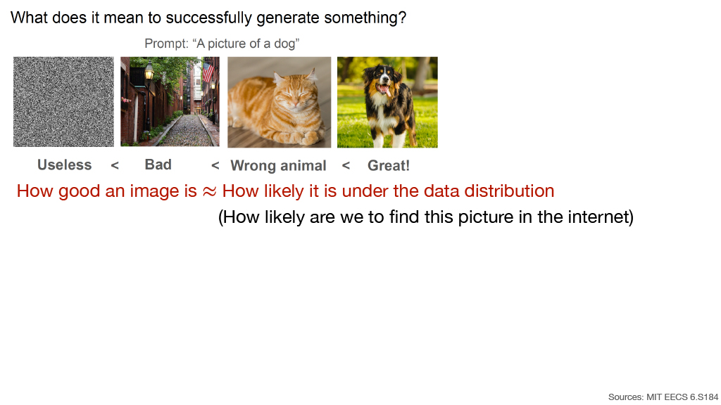
Slide 7-8: What Does Successful Generation Mean?

Example prompt:

“A picture of a dog”

The slide compares four outputs:

Random noise — Useless
An unrelated street image — Bad
A cat image — Wrong animal
A dog image — Great!

The central intuition is:

How good an image is ≈ How likely it is under the data distribution.

Another interpretation:

How likely are we to find this picture on the internet?

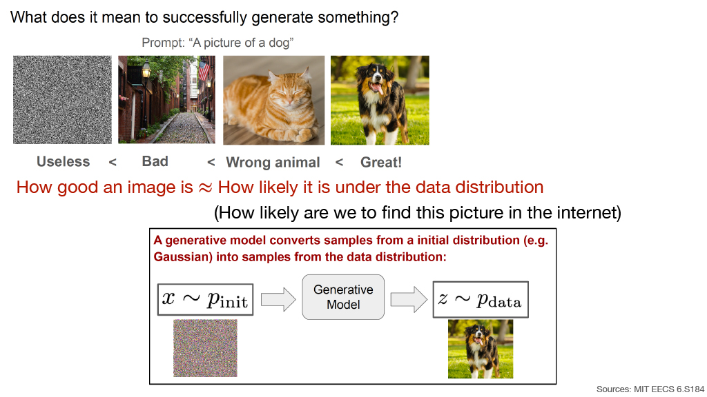
A generative model converts samples from a simple initial distribution, such as a Gaussian distribution, into samples resembling the data distribution.

$$ x\sim p_{\text{init}} \quad \xrightarrow{\text{Generative Model}} \quad z\sim p_{\text{data}}. $$

The initial sample is visualized as noise.
The final sample is visualized as a realistic dog image.
Source: MIT EECS 6.S184

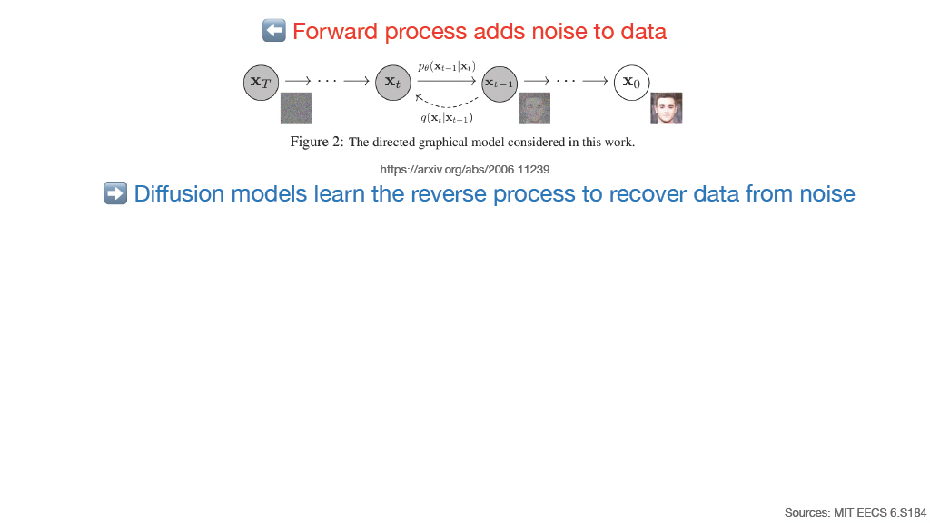
Slide 9-10: Forward and Reverse Diffusion Processes

Reference:

https://arxiv.org/abs/2006.11239

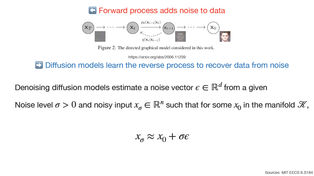
The DDPM graphical model illustrates a sequence from clean data $x_0$ toward increasingly noisy states $x_1,\ldots,x_T$.

⬅ Forward process adds noise to data
➡ Diffusion models learn the reverse process to recover data from noise

Denoising diffusion models estimate a noise vector

$$ \epsilon\in\mathbb{R}^d $$

from a given noise level

$$ \sigma>0 $$

and noisy input

$$ x_\sigma\in\mathbb{R}^n, $$

such that, for some clean point $x_0$ on the data manifold $\mathcal K$,

$$ x_\sigma \approx x_0+\sigma\epsilon. $$

Source: MIT EECS 6.S184

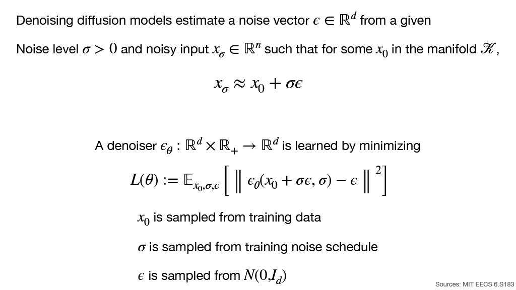
Slide 11: Learning a Noise Predictor

A denoiser is represented as

$$ \epsilon_\theta:\mathbb{R}^d\times\mathbb{R}_+\rightarrow\mathbb{R}^d. $$

It is trained by minimizing the expected noise-prediction error:

$$ L(\theta) := \mathbb{E}_{x_0,\sigma,\epsilon} \left[ \left\| \epsilon_\theta(x_0+\sigma\epsilon,\sigma)-\epsilon \right\|_2^2 \right]. $$

During training:

$x_0$ is sampled from the training data.
$\sigma$ is sampled from the training noise schedule.
$\epsilon$ is sampled from a standard Gaussian distribution:

$$ \epsilon\sim\mathcal N(0,I_d). $$

The noisy input given to the model is therefore

$$ x_\sigma=x_0+\sigma\epsilon. $$

Source: MIT EECS 6.S183

Slide 12: 2. Algorithms

Section 2 describes concrete training and sampling algorithms for a simple diffusion model.

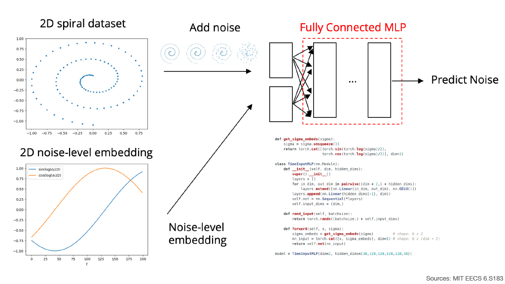
Slide 13: A Toy 2D Diffusion Model

The model is demonstrated using a 2D spiral dataset.

Pipeline:

Start with points on a 2D spiral.
Add different amounts of Gaussian noise.
Embed the noise level.
Feed both the noisy point and noise-level embedding into a fully connected MLP.
Predict the noise.

The noise-level embedding is two-dimensional and is visualized using sinusoidal functions:

$$ \sin\left(\frac{\log(\sigma_t)}{2}\right), \qquad \cos\left(\frac{\log(\sigma_t)}{2}\right). $$

The slide contains the following model implementation:

def get_sigma_embeds(sigma):
    sigma = sigma.unsqueeze(1)
    return torch.cat([
        torch.sin(torch.log(sigma) / 2),
        torch.cos(torch.log(sigma) / 2)
    ], dim=1)


class TimeInputMLP(nn.Module):
    def __init__(self, dim, hidden_dims):
        super().__init__()
        layers = []

        for in_dim, out_dim in pairwise((dim + 2,) + hidden_dims):
            layers.extend([nn.Linear(in_dim, out_dim), nn.GELU()])

        layers.append(nn.Linear(hidden_dims[-1], dim))
        self.net = nn.Sequential(*layers)
        self.input_dims = (dim,)

    def rand_input(self, batchsize):
        return torch.randn((batchsize,) + self.input_dims)

    def forward(self, x, sigma):
        sigma_embeds = get_sigma_embeds(sigma)  # shape: b x 2
        nn_input = torch.cat([x, sigma_embeds], dim=1)  # shape: b x (dim + 2)
        return self.net(nn_input)


model = TimeInputMLP(
    dim=2,
    hidden_dims=(16, 128, 128, 128, 128, 16)
)

Source: MIT EECS 6.S183

Slide 14: Training the Noise-Prediction Model

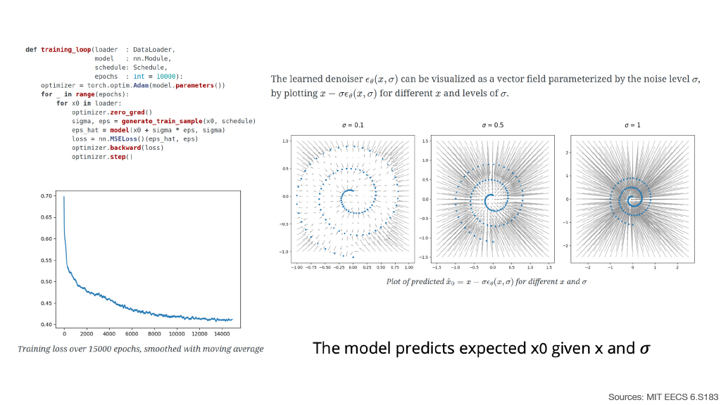
The training loop repeatedly generates noisy samples and minimizes mean squared error between predicted and true noise.

def training_loop(loader: DataLoader,
                  model: nn.Module,
                  schedule: Schedule,
                  epochs: int = 10000):

    optimizer = torch.optim.Adam(model.parameters())

    for _ in range(epochs):
        for x0 in loader:
            optimizer.zero_grad()

            sigma, eps = generate_train_sample(x0, schedule)

            eps_hat = model(x0 + sigma * eps, sigma)

            loss = nn.MSELoss()(eps_hat, eps)

            optimizer.backward(loss)
            optimizer.step()

The slide shows the training loss over approximately 15,000 epochs, smoothed using a moving average. The loss gradually decreases during training.

The learned denoiser

$$ \epsilon_\theta(x,\sigma) $$

can be visualized as a vector field parameterized by the noise level $\sigma$.

The visualization plots

$$ x-\sigma\epsilon_\theta(x,\sigma) $$

for different $x$ and different values of $\sigma$:

$\sigma=0.1$
$\sigma=0.5$
$\sigma=1$

The central interpretation is:

The model predicts expected $x_0$ given $x$ and $\sigma$.

Source: MIT EECS 6.S183

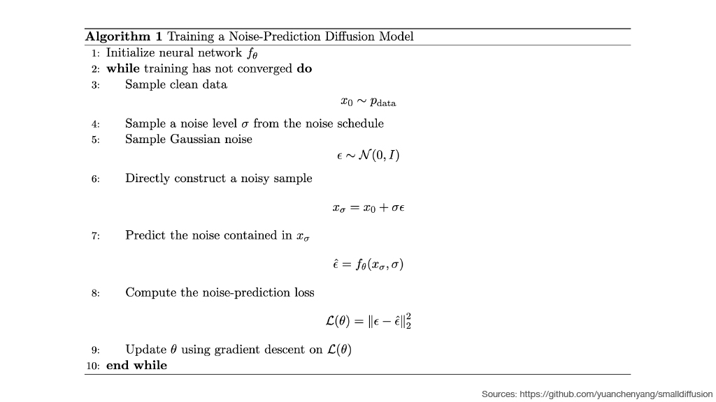
Slide 15: Algorithm 1 — Training a Noise-Prediction Diffusion Model

Algorithm 1: Training a Noise-Prediction Diffusion Model

Initialize neural network $f_\theta$.
While training has not converged:
Sample clean data:

$$ x_0\sim p_{\text{data}}. $$

Sample a noise level $\sigma$ from the noise schedule.
Sample Gaussian noise:

$$ \epsilon\sim\mathcal N(0,I). $$

Directly construct a noisy sample:

$$ x_\sigma=x_0+\sigma\epsilon. $$

Predict the noise contained in $x_\sigma$:

$$ \hat{\epsilon}=f_\theta(x_\sigma,\sigma). $$

Compute the noise-prediction loss:

$$ \mathcal L(\theta) = \|\epsilon-\hat{\epsilon}\|_2^2. $$

Update $\theta$ using gradient descent on $\mathcal L(\theta)$.
End while.

Source: https://github.com/yuanchenyang/smalldiffusion

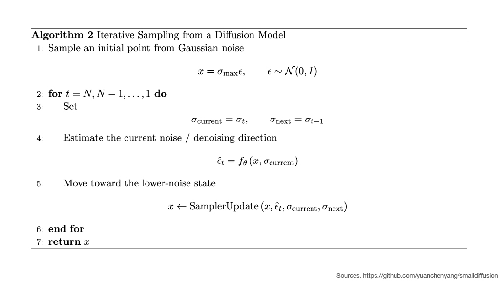
Slide 16: Algorithm 2 — Iterative Sampling from a Diffusion Model

Algorithm 2: Iterative Sampling from a Diffusion Model

Sample an initial point from Gaussian noise:

$$ x=\sigma_{\max}\epsilon, \qquad \epsilon\sim\mathcal N(0,I). $$

$$ t=N,N-1,\ldots,1 $$

do:

$$ \sigma_{\text{current}}=\sigma_t, \qquad \sigma_{\text{next}}=\sigma_{t-1}. $$

Estimate the current noise / denoising direction:

$$ \hat{\epsilon}_t = f_\theta(x,\sigma_{\text{current}}). $$

Move toward the lower-noise state:

$$ x \leftarrow \operatorname{SamplerUpdate} \left( x, \hat{\epsilon}_t, \sigma_{\text{current}}, \sigma_{\text{next}} \right). $$

End for.
Return $x$.

Source: https://github.com/yuanchenyang/smalldiffusion

Slide 17: 3. Training Details

Section 3 examines the mathematical structure of the optimal denoiser learned by the noise-prediction objective.

Slide 18: The Ideal Denoiser

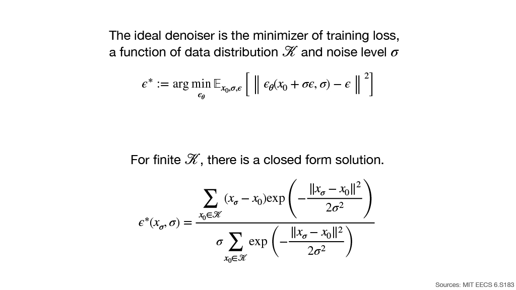
The ideal denoiser is defined as the minimizer of the training objective:

$$ \epsilon^* := \arg\min_{\epsilon_\theta} \mathbb{E}_{x_0,\sigma,\epsilon} \left[ \left\| \epsilon_\theta(x_0+\sigma\epsilon,\sigma)-\epsilon \right\|_2^2 \right]. $$

For a finite dataset or manifold representation $\mathcal K$, the optimal predictor has a closed-form solution:

$$ \epsilon^*(x_\sigma,\sigma) = \frac{ \displaystyle \sum_{x_0\in\mathcal K} (x_\sigma-x_0) \exp\left( -\frac{\|x_\sigma-x_0\|^2}{2\sigma^2} \right) }{ \displaystyle \sigma \sum_{x_0\in\mathcal K} \exp\left( -\frac{\|x_\sigma-x_0\|^2}{2\sigma^2} \right) }. $$

Key points:

The ideal denoiser is the minimizer of the training loss.
It is a function of both the data distribution $\mathcal K$ and the noise level $\sigma$.
For finite $\mathcal K$, there is a closed-form solution.
Source: MIT EECS 6.S183

Slide 19: Denoising Vector Fields at Different Noise Levels

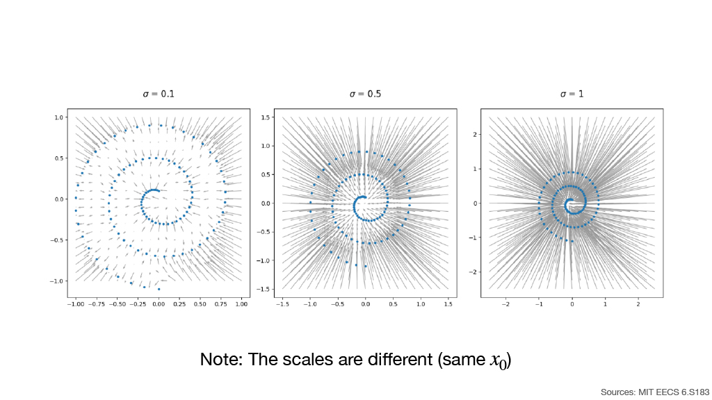
The slide visualizes the predicted denoising direction for the same underlying $x_0$ using three noise levels:

$\sigma=0.1$
$\sigma=0.5$
$\sigma=1$

As $\sigma$ increases:

The region being considered becomes larger.
The denoising vectors aggregate information over a broader neighborhood of the data manifold.
For small $\sigma$, the denoising direction is much more local.

Note: The scales are different (same $x_0$).

Source: MIT EECS 6.S183

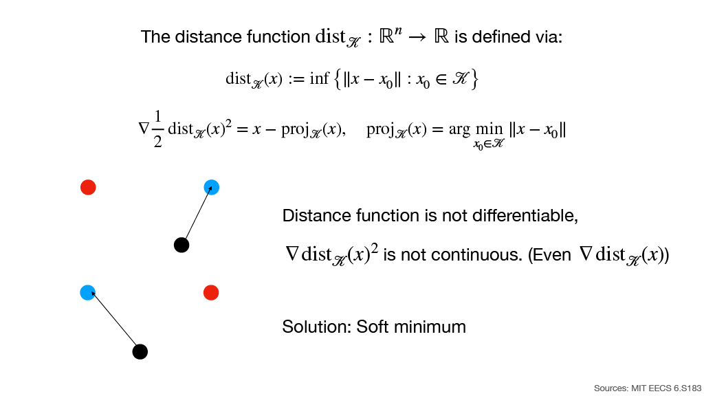
Slide 20-21: Distance to the Data Manifold

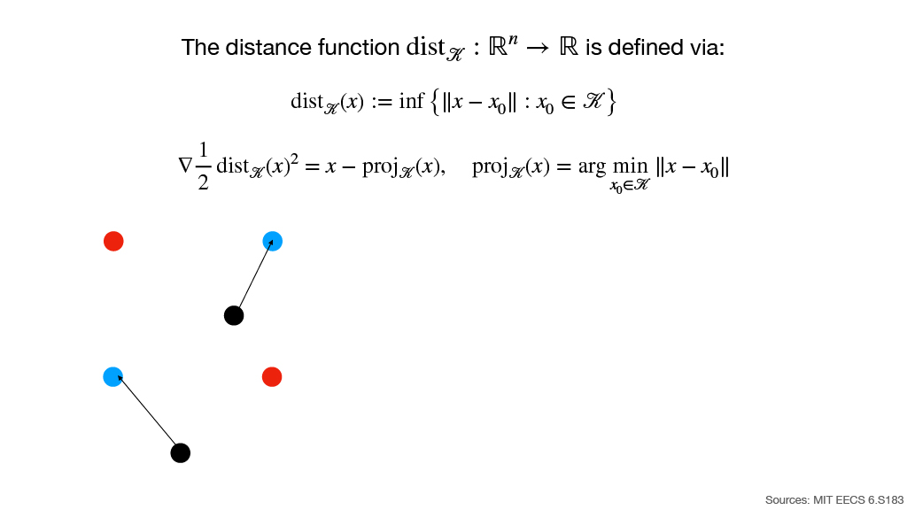
The distance function

$$ \operatorname{dist}_{\mathcal K}:\mathbb{R}^n\rightarrow\mathbb{R} $$

is defined as

$$ \operatorname{dist}_{\mathcal K}(x) := \inf \left\{ \|x-x_0\|:x_0\in\mathcal K \right\}. $$

The gradient of the squared distance is related to projection onto the data manifold:

$$ \nabla \frac{1}{2} \operatorname{dist}_{\mathcal K}(x)^2 = x-\operatorname{proj}_{\mathcal K}(x), $$

where

$$ \operatorname{proj}_{\mathcal K}(x) = \arg\min_{x_0\in\mathcal K} \|x-x_0\|. $$

However, this construction causes a problem:

The distance function is not differentiable everywhere.
$\nabla\operatorname{dist}_{\mathcal K}(x)^2$ is not continuous.

The proposed solution is:

Soft minimum

Source: MIT EECS 6.S183

Slide 22-23: Gaussian-Smoothed Distance Function

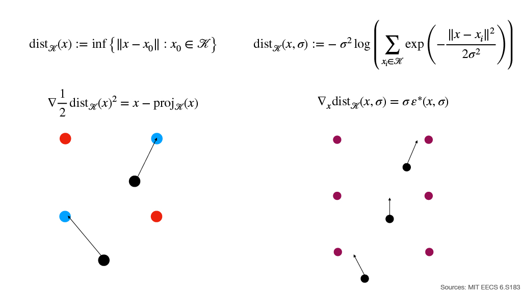
Instead of the hard minimum, define a smooth approximation:

$$ \operatorname{dist}_{\mathcal K}(x,\sigma) := -\sigma^2 \log \sum_{x_i\in\mathcal K} \exp \left( -\frac{\|x-x_i\|^2}{2\sigma^2} \right). $$

Its gradient satisfies

$$ \nabla_x \operatorname{dist}_{\mathcal K}(x,\sigma) = \sigma\epsilon^*(x,\sigma). $$

For comparison, the original hard distance was

$$ \operatorname{dist}_{\mathcal K}(x) := \inf \left\{ \|x-x_0\|:x_0\in\mathcal K \right\}, $$

with

$$ \nabla \frac12 \operatorname{dist}_{\mathcal K}(x)^2 = x-\operatorname{proj}_{\mathcal K}(x). $$

Therefore:

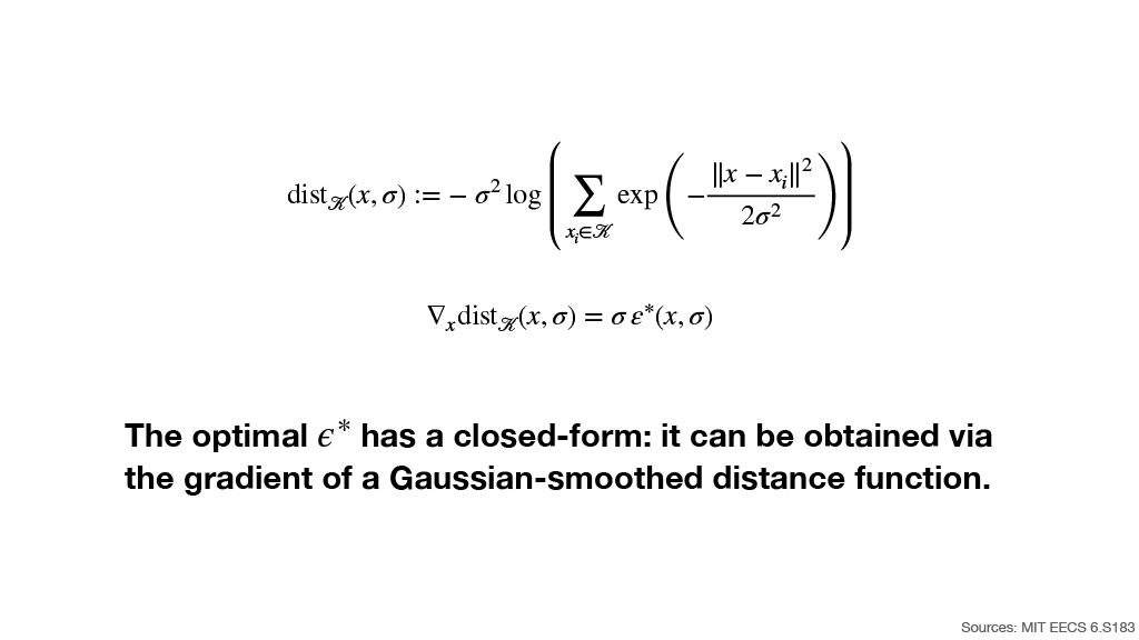
The optimal $\epsilon^*$ has a closed form: it can be obtained via the gradient of a Gaussian-smoothed distance function.

Source: MIT EECS 6.S183

Slide 24: 4. Sampling Details

Section 4 explains how the trained denoiser is used to iteratively move a noisy sample toward the data distribution.

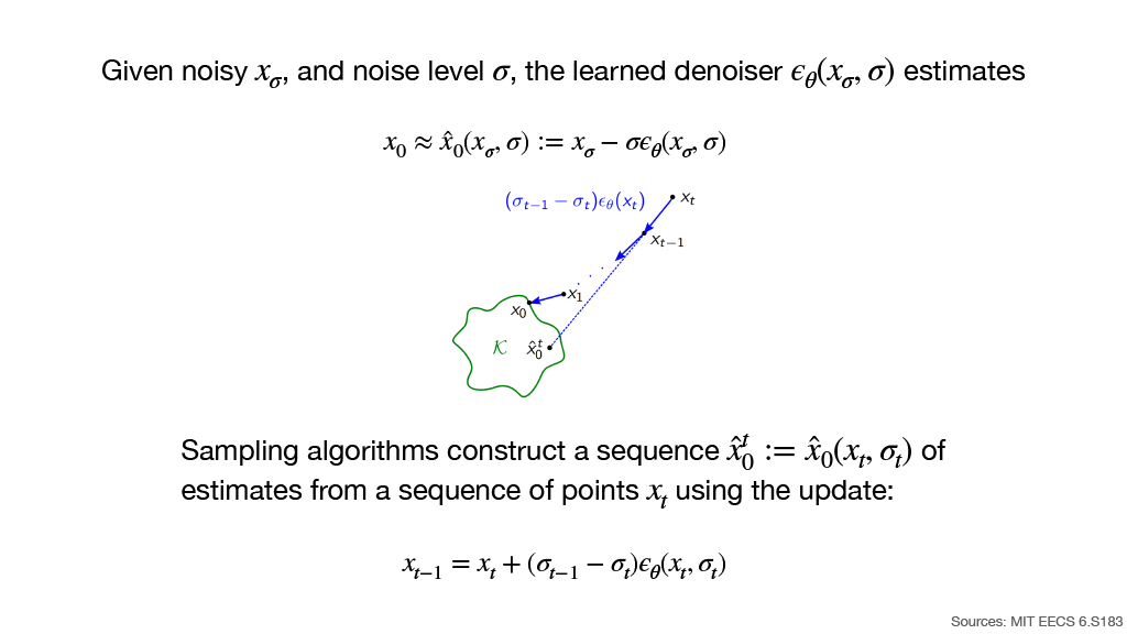
Slide 25: From Noise Prediction to a Clean-Data Estimate

Given noisy $x_\sigma$ and noise level $\sigma$, the learned denoiser predicts

$$ \epsilon_\theta(x_\sigma,\sigma). $$

This produces an estimate of the underlying clean sample:

$$ x_0 \approx \hat{x}_0(x_\sigma,\sigma) := x_\sigma-\sigma\epsilon_\theta(x_\sigma,\sigma). $$

The diagram visualizes:

The current noisy point $x_t$.
An estimate $\hat{x}_0^t$ on or near the data manifold $\mathcal K$.
The next point $x_{t-1}$, obtained by moving along the predicted denoising direction.
Repeating this process progressively approaches the manifold.

Sampling algorithms construct a sequence of clean-data estimates

$$ \hat{x}_0^t := \hat{x}_0(x_t,\sigma_t) $$

from a sequence $x_t$ using

$$ x_{t-1} = x_t + (\sigma_{t-1}-\sigma_t) \epsilon_\theta(x_t,\sigma_t). $$

Source: MIT EECS 6.S183

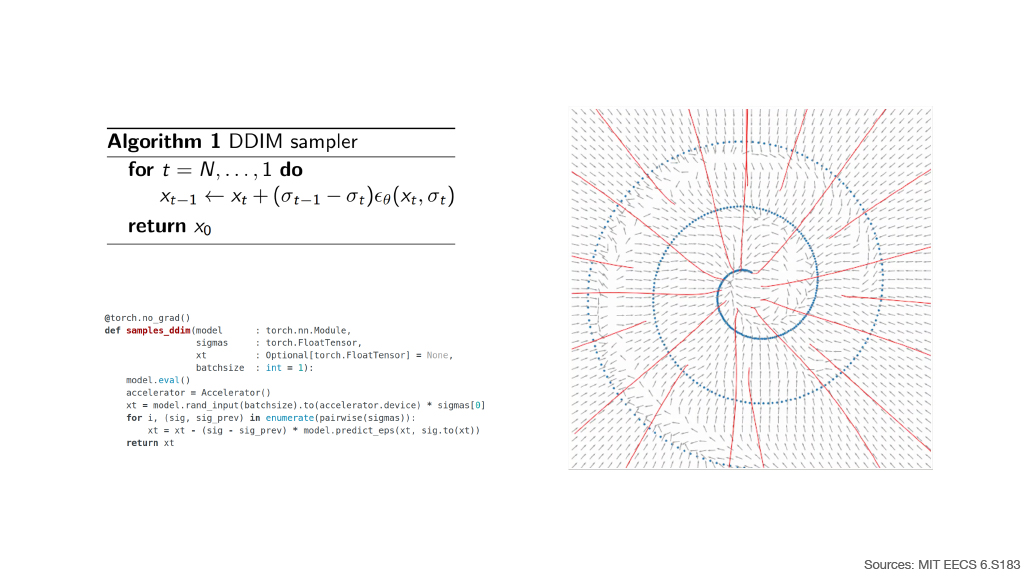
Slide 26: DDIM Sampler

The DDIM sampler repeatedly applies the deterministic update

$$ x_{t-1} \leftarrow x_t + (\sigma_{t-1}-\sigma_t) \epsilon_\theta(x_t,\sigma_t). $$

Algorithm:

Algorithm 1 DDIM sampler

for t = N, ..., 1 do
    x_{t-1} ← x_t + (σ_{t-1} - σ_t) ε_θ(x_t, σ_t)

return x_0

The slide also contains an implementation of the sampler and a vector-field visualization.

The red sampling trajectories start from high-noise regions and iteratively follow the denoising vector field toward the spiral-shaped data manifold.

Source: MIT EECS 6.S183

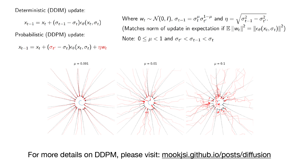
Slide 27: Deterministic DDIM vs. Probabilistic DDPM

Deterministic DDIM Update

$$ x_{t-1} = x_t + (\sigma_{t-1}-\sigma_t) \epsilon_\theta(x_t,\sigma_t). $$

Probabilistic DDPM Update

$$ x_{t-1} = x_t + (\sigma_{t'}-\sigma_t) \epsilon_\theta(x_t,\sigma_t) + \eta w_t. $$

where

$$ w_t\sim\mathcal N(0,I), $$

$$ \sigma_{t-1} = \sigma_t^\mu \sigma_{t'}^{\,1-\mu}, $$

and

$$ \eta = \sqrt{ \sigma_{t-1}^2-\sigma_{t'}^2 }. $$

The noise scale is chosen so that the norm of the stochastic update matches the denoising update in expectation when

$$ \mathbb{E}\|w_t\|^2 = \|\epsilon_\theta(x_t,\sigma_t)\|^2. $$

The slide notes:

$$ 0\le\mu<1, \qquad \sigma_{t'}<\sigma_{t-1}<\sigma_t. $$

Three visual examples compare sampling trajectories for:

$\mu=0.001$
$\mu=0.01$
$\mu=0.1$

As $\mu$ increases, the trajectories become progressively more stochastic.

For more details on DDPM, please visit: mookjsi.github.io/posts/diffusion

Slide 28: 5. Conditional Sampling

Section 5 extends unconditional diffusion models to conditional generation.

Slide 29: How Can We Sample Conditionally?

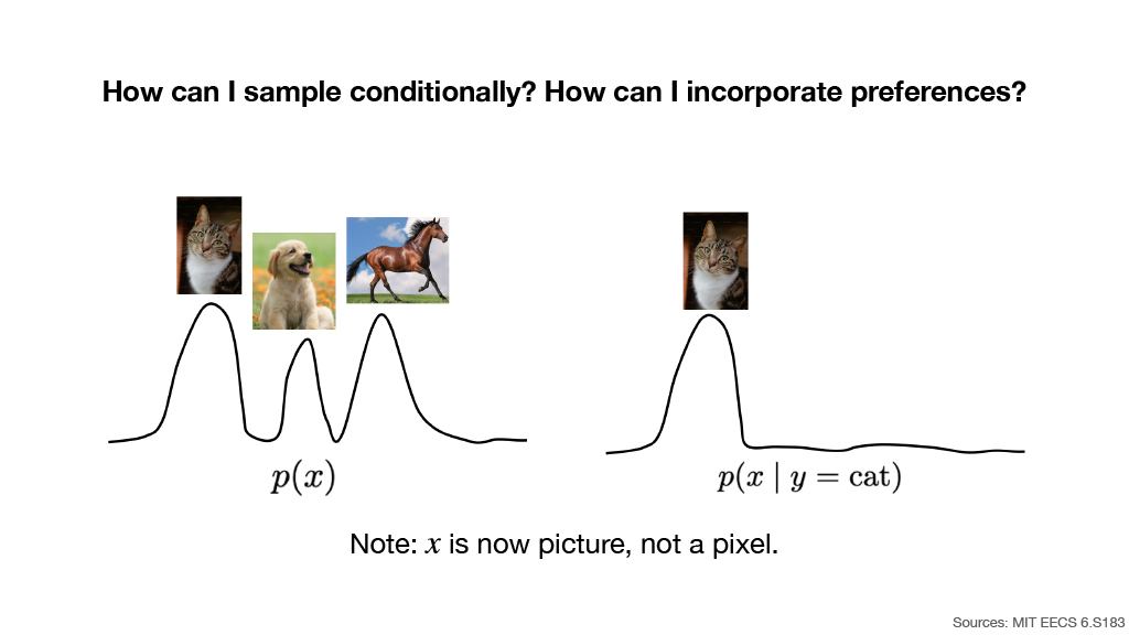
The main questions are:

How can I sample conditionally? How can I incorporate preferences?

The slide contrasts:

$$ p(x) $$

with a conditional distribution such as

$$ p(x\mid y=\text{cat}). $$

The unconditional distribution contains several types of images, including:

Cat
Dog
Horse

Conditioning on $y=\text{cat}$ restricts generation toward the cat mode.

Note: $x$ is now a picture, not a pixel.

Source: MIT EECS 6.S183

Slide 30: Conditional Score Matching

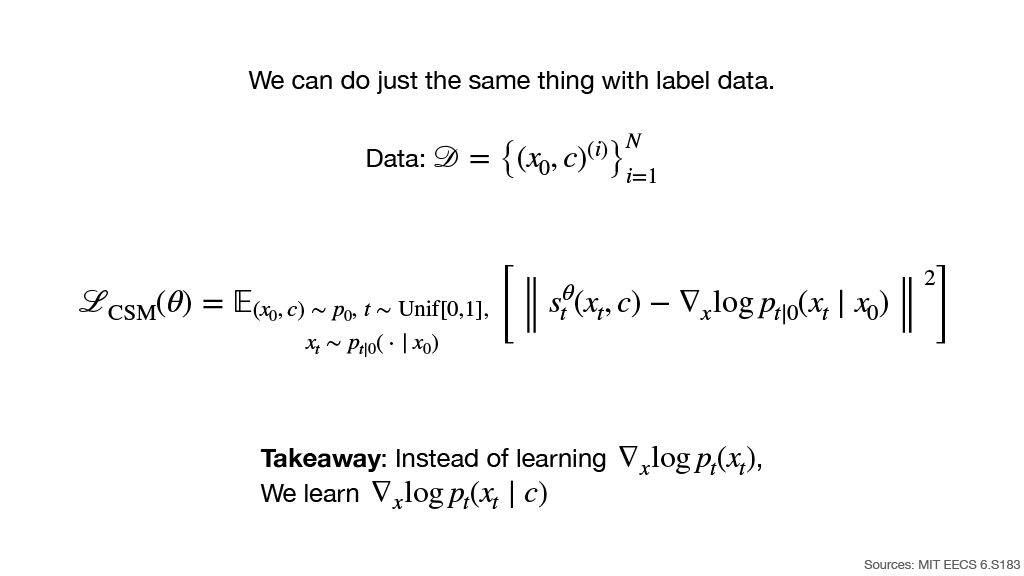
The same idea can be applied when labels are available.

Dataset:

$$ \mathcal D = \left\{ (x_0,c)^{(i)} \right\}_{i=1}^{N}. $$

The conditional score-matching objective is

$$ \mathcal L_{\mathrm{CSM}}(\theta) = \mathbb E_{ (x_0,c)\sim p_0,\; t\sim\mathrm{Unif}[0,1],\; x_t\sim p_{t|0}(\cdot|x_0) } \left[ \left\| s_t^\theta(x_t,c) - \nabla_x \log p_{t|0}(x_t|x_0) \right\|^2 \right]. $$

The key takeaway is that instead of learning the unconditional score

$$ \nabla_x\log p_t(x_t), $$

we learn the conditional score

$$ \nabla_x\log p_t(x_t\mid c). $$

Source: MIT EECS 6.S183

Slide 31: Conditional and Unconditional ODE Flows

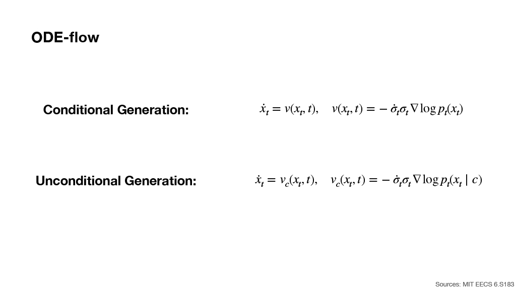
Unconditional Generation

$$ \dot{x}_t = v(x_t,t), $$

where

$$ v(x_t,t) = -\dot{\sigma}_t \sigma_t \nabla\log p_t(x_t). $$

Conditional Generation

$$ \dot{x}_t = v_c(x_t,t), $$

where

$$ v_c(x_t,t) = -\dot{\sigma}_t \sigma_t \nabla\log p_t(x_t\mid c). $$

Thus, conditional generation modifies the ODE vector field by replacing the unconditional score with the conditional score.

Source: MIT EECS 6.S183

Slide 32: 6. Latent Diffusion Models

Section 6 introduces latent diffusion, where the diffusion process is performed in a lower-dimensional latent representation rather than directly in image space.

Slide 33-34: Latent Diffusion Models — Algorithm

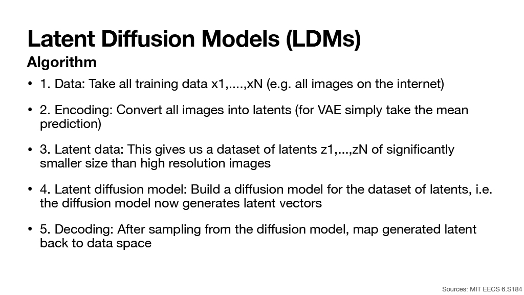
The latent diffusion pipeline consists of five steps.

Data
Take all training data

$$ x_1,\ldots,x_N $$

such as images collected from the internet.

Encoding
Convert all images into latent representations.
- For a VAE, simply take the mean prediction.
Latent Data
This creates a new dataset

$$ z_1,\ldots,z_N, $$

whose elements are significantly smaller than the original high-resolution images.

Latent Diffusion Model
Build a diffusion model on the dataset of latent variables.
- The diffusion model now generates latent vectors instead of full-resolution images.
Decoding
After sampling from the diffusion model, map the generated latent representation back into the original data space.

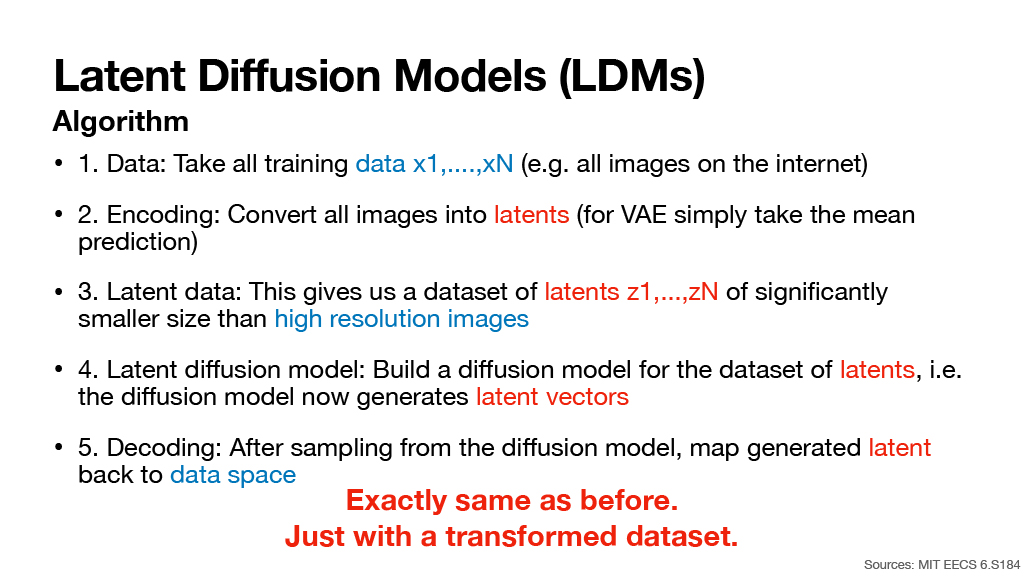
The central message of Slide 34 is:

Exactly same as before. Just with a transformed dataset.

Source: MIT EECS 6.S184

Slide 35: Why Generate in Latent Space?

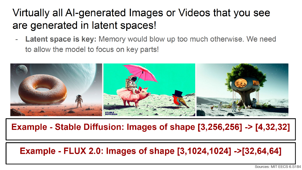
The slide states:

Virtually all AI-generated images or videos that you see are generated in latent spaces!

Why?

Latent space is key because memory usage would otherwise become prohibitively large.
A compressed representation also allows the model to focus on important components of the data.

Examples:

Stable Diffusion

Original image representation:

$$ [3,256,256] $$

is compressed to:

$$ [4,32,32]. $$

FLUX 2.0

Original image representation:

$$ [3,1024,1024] $$

is compressed to:

$$ [32,64,64]. $$

The slide includes three examples of AI-generated imagery to illustrate high-resolution generation from latent representations.

Source: MIT EECS 6.S184

Slide 36: Parameterizing a Vector Field in a Neural Network

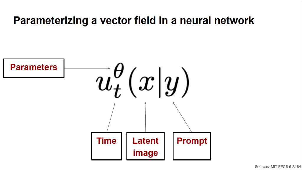
A diffusion model can parameterize a vector field using a neural network:

$$ u_t^\theta(x\mid y). $$

The network depends on three principal inputs:

Time
Latent image
Prompt

The network parameters are represented by $\theta$.

The diagram therefore expresses a conditional vector field whose behavior depends jointly on:

the current diffusion time,
the current image latent,
and the text condition.
Source: MIT EECS 6.S184

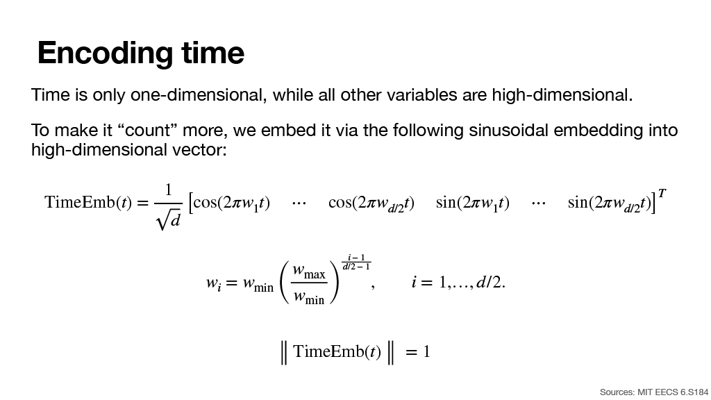
Slide 37: Encoding Time

Time is only one-dimensional, while the other model variables are high-dimensional.

To make the time variable “count” more, it is embedded into a high-dimensional vector using sinusoidal features.

$$ \operatorname{TimeEmb}(t) = \frac{1}{\sqrt d} \begin{bmatrix} \cos(2\pi w_1t) & \cdots & \cos(2\pi w_{d/2}t) & \sin(2\pi w_1t) & \cdots & \sin(2\pi w_{d/2}t) \end{bmatrix}^{T}. $$

The frequencies are geometrically spaced:

$$ w_i = w_{\min} \left( \frac{w_{\max}}{w_{\min}} \right)^{ \frac{i-1}{d/2-1} }, \qquad i=1,\ldots,d/2. $$

The embedding is normalized:

$$ \left\| \operatorname{TimeEmb}(t) \right\| = 1. $$

Source: MIT EECS 6.S184

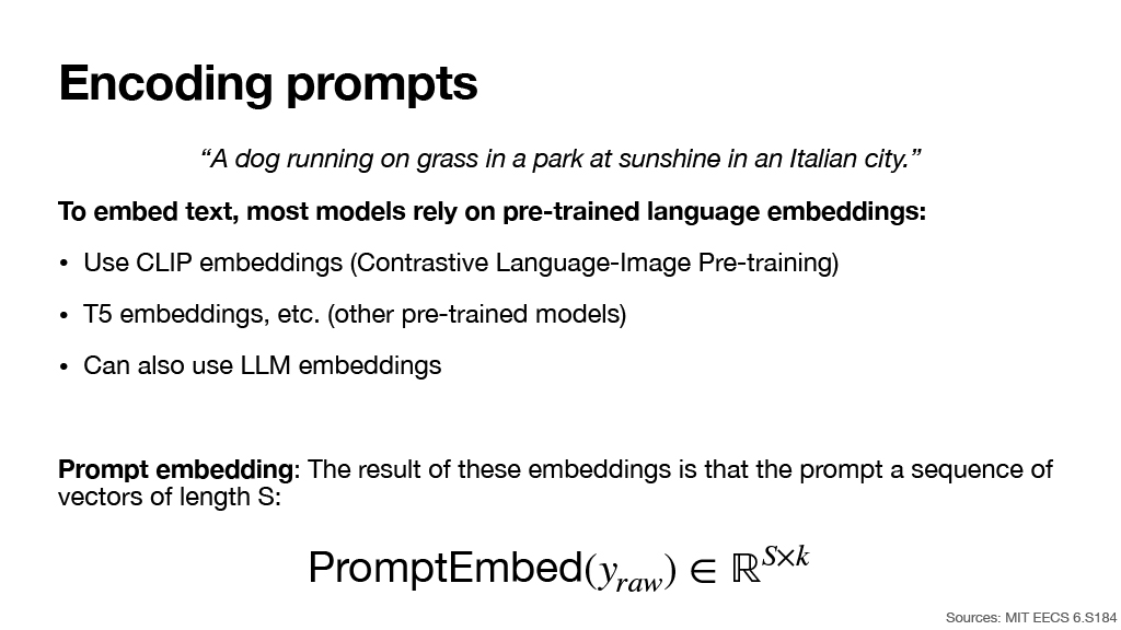
Slide 38: Encoding Prompts

Example prompt:

“A dog running on grass in a park at sunshine in an Italian city.”

Most generative models embed text using pre-trained language or multimodal representations.

Possible choices include:

CLIP embeddings
- Contrastive Language-Image Pre-training
T5 embeddings
Other pre-trained models
LLM embeddings

The result is a sequence of $S$ vectors:

$$ \operatorname{PromptEmbed}(y_{\mathrm{raw}}) \in \mathbb{R}^{S\times k}. $$

Here:

$S$ is the sequence length.
$k$ is the dimensionality of each token embedding.
Source: MIT EECS 6.S184

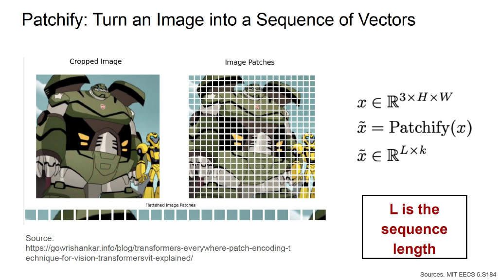
Slide 39: Patchify — Turn an Image into a Sequence of Vectors

Transformers operate naturally on sequences. Therefore, an image can be divided into patches and represented as a sequence.

The original image is represented as

$$ x\in\mathbb{R}^{3\times H\times W}. $$

Patchification produces

$$ \tilde{x} = \operatorname{Patchify}(x), $$

with

$$ \tilde{x} \in \mathbb{R}^{L\times k}. $$

where:

$L$ is the sequence length.
$k$ is the dimensionality of each patch vector.

The slide visually shows:

A cropped image.
The image divided into a rectangular patch grid.
The patches flattened into a one-dimensional sequence of vectors.

Image source shown on the slide:

https://glorivishankar.info/blog/transformers-everywhere-patch-encoding-technique-for-vision-transformers-vit-explained/
Source: MIT EECS 6.S184

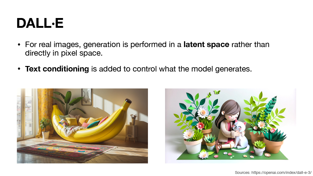
Slide 40: DALL·E

For real images:

Generation is performed in a latent space rather than directly in pixel space.
Text conditioning is added to control what the model generates.

The slide shows two examples of generated images:

A surreal banana-shaped hammock placed inside a room.
A stylized character surrounded by flowers and plants.

These examples illustrate text-conditioned image synthesis.

Source: https://openai.com/index/dall-e-3/

Slide 41: Diffusion Transformer (DiT)

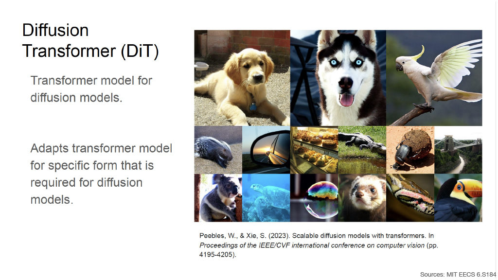
Diffusion Transformer (DiT)

A Transformer model designed for diffusion models.
It adapts the Transformer architecture to the specific form required by diffusion models.

The slide shows a collection of generated animal images.

Reference shown on the slide:

Peebles, W., & Xie, S. (2023). Scalable diffusion models with transformers.
Proceedings of the IEEE/CVF International Conference on Computer Vision, pp. 4195–4205.

Source: MIT EECS 6.S184

Slide 42: MovieGen

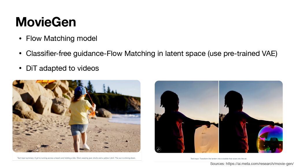
MovieGen combines several of the previously introduced ideas.

Flow Matching model
Classifier-free guidance
Flow Matching is performed in latent space
- A pre-trained VAE is used.
DiT adapted to videos

The slide shows examples from MovieGen:

A generated video of a person running along a beach or rocky coastal environment.
A video-editing example in which the appearance/content of an object held by a person is modified across frames.
Source: https://ai.meta.com/research/movie-gen/

Slide 43: Sora

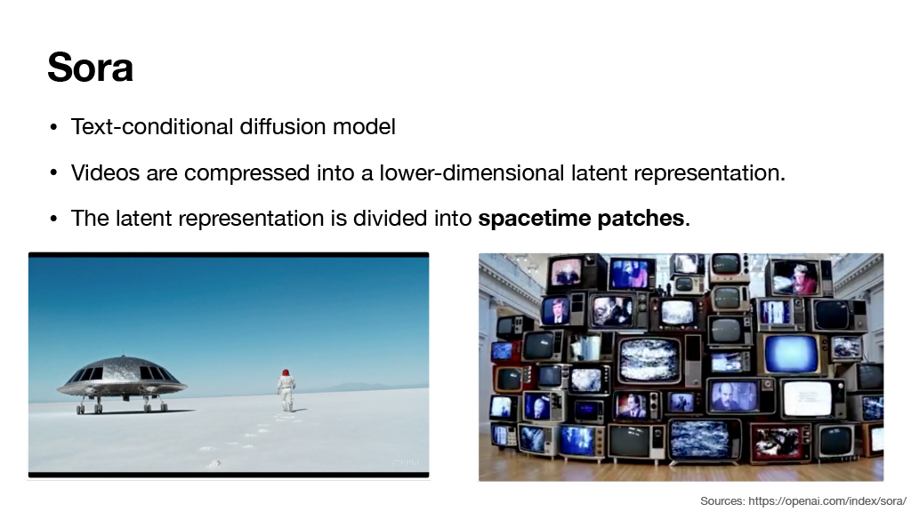
Sora extends the diffusion-model framework to video generation.

Text-conditional diffusion model
Videos are compressed into a lower-dimensional latent representation.
The latent representation is divided into spacetime patches.

This combines three major ideas introduced earlier:

Conditional generation
- Text controls the output.
Latent diffusion
- Generation occurs in a compressed representation instead of full pixel space.
Patch-based Transformer processing
- Video latents are divided into spacetime patches that can be processed as tokens.

The slide contains two Sora examples:

A surreal outdoor scene containing a large futuristic or spacecraft-like object.
A composition consisting of many televisions/screens displaying different visual content.
Source: https://openai.com/index/sora/