Slide 1: Preface
- Topic: Diffusion Models (In Process)
- Sources referenced:
- Deep Generative Modeling, Jacob M. Tomczak, 2022
- Denoising Diffusion Probabilistic Models, Ho et al., 2020
- Deep Unsupervised Learning using Nonequilibrium Thermodynamics, Sohl-Dickstein et al., 2015
Slide 2: Introduction - Data Representation
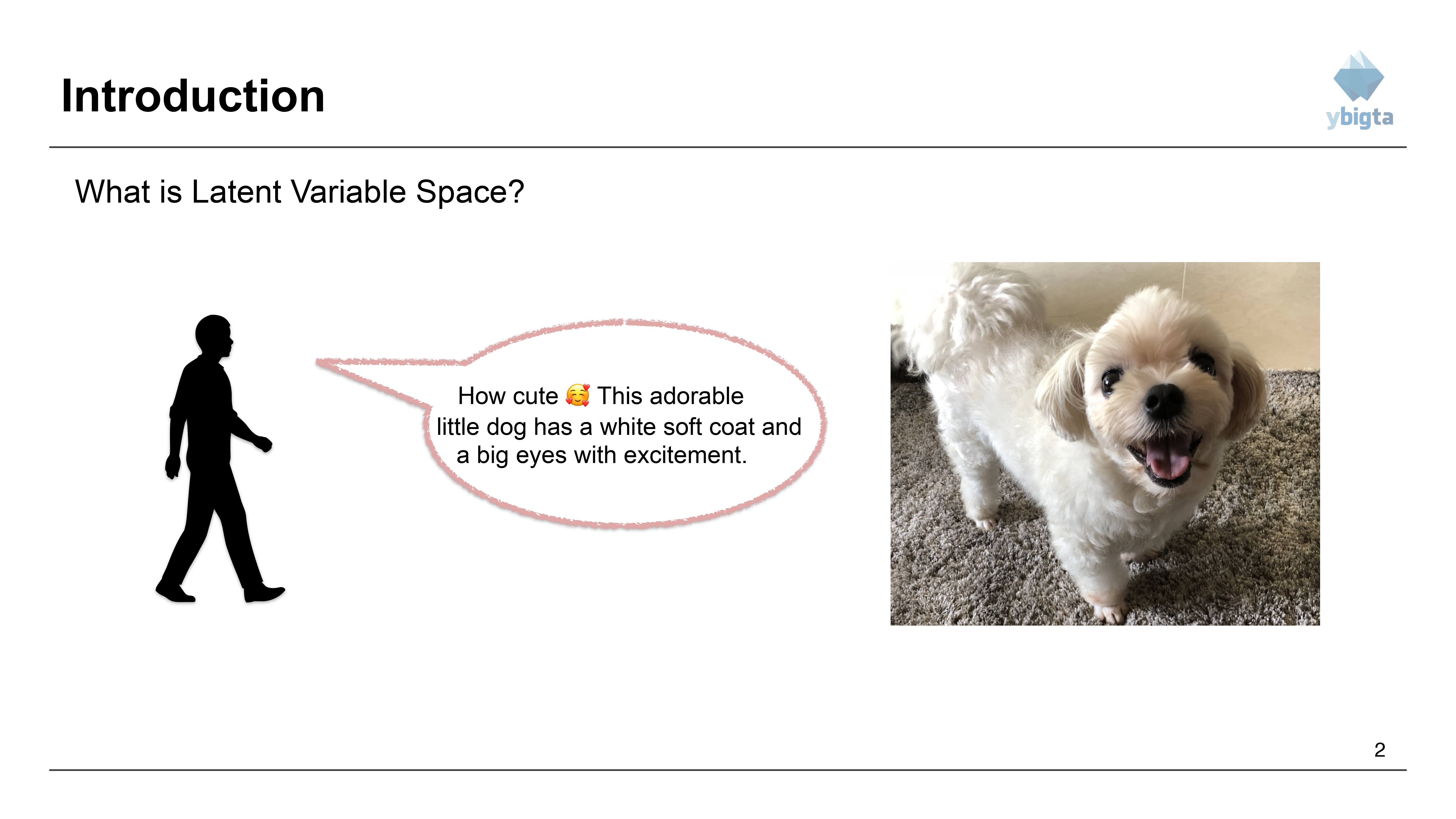
- An example of how we perceive data versus how a machine might process features.
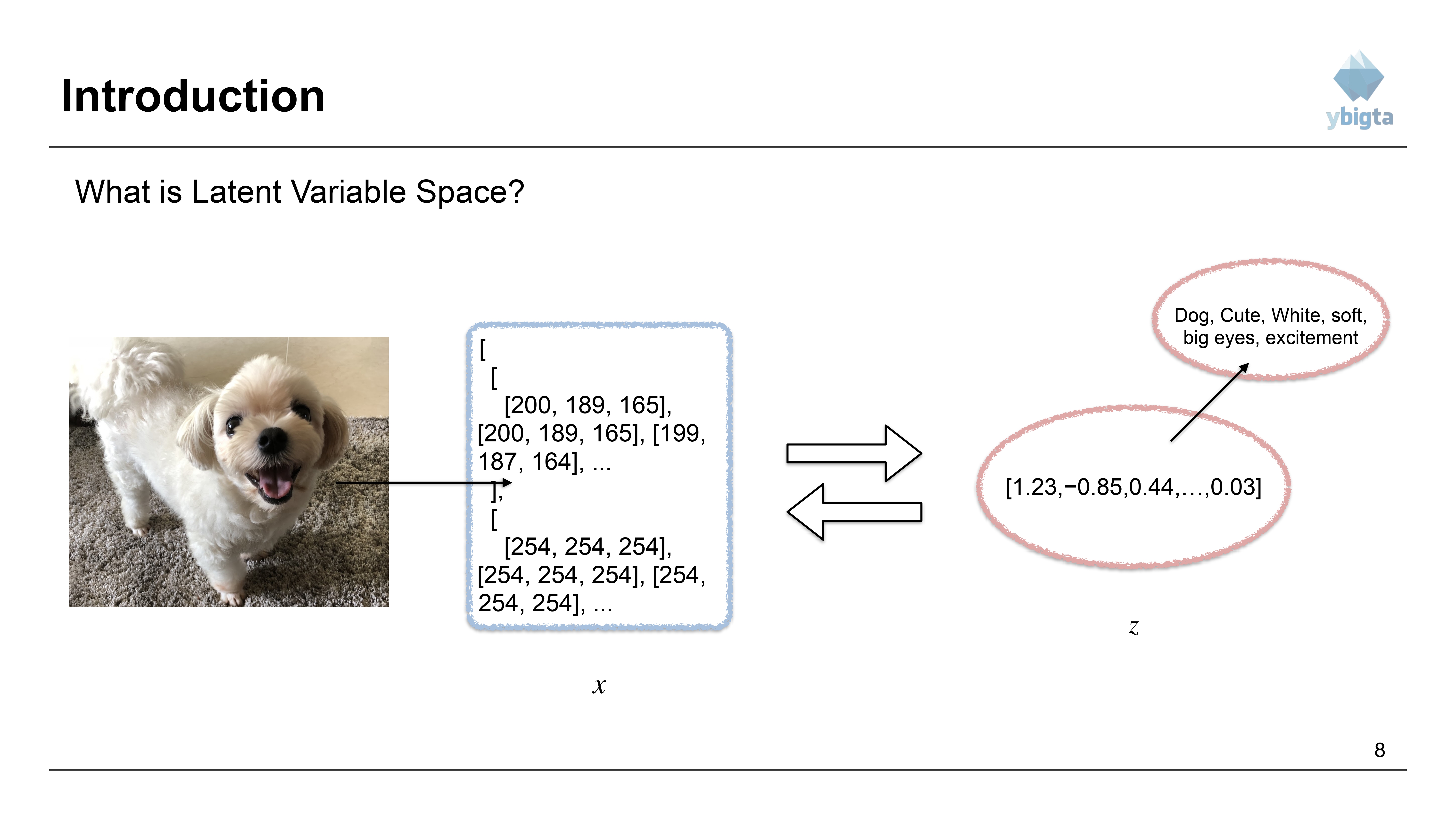
- Human view: “How cute! This adorable little dog has a white soft coat and big eyes with excitement.”
- Visual Data: An image of a white dog.
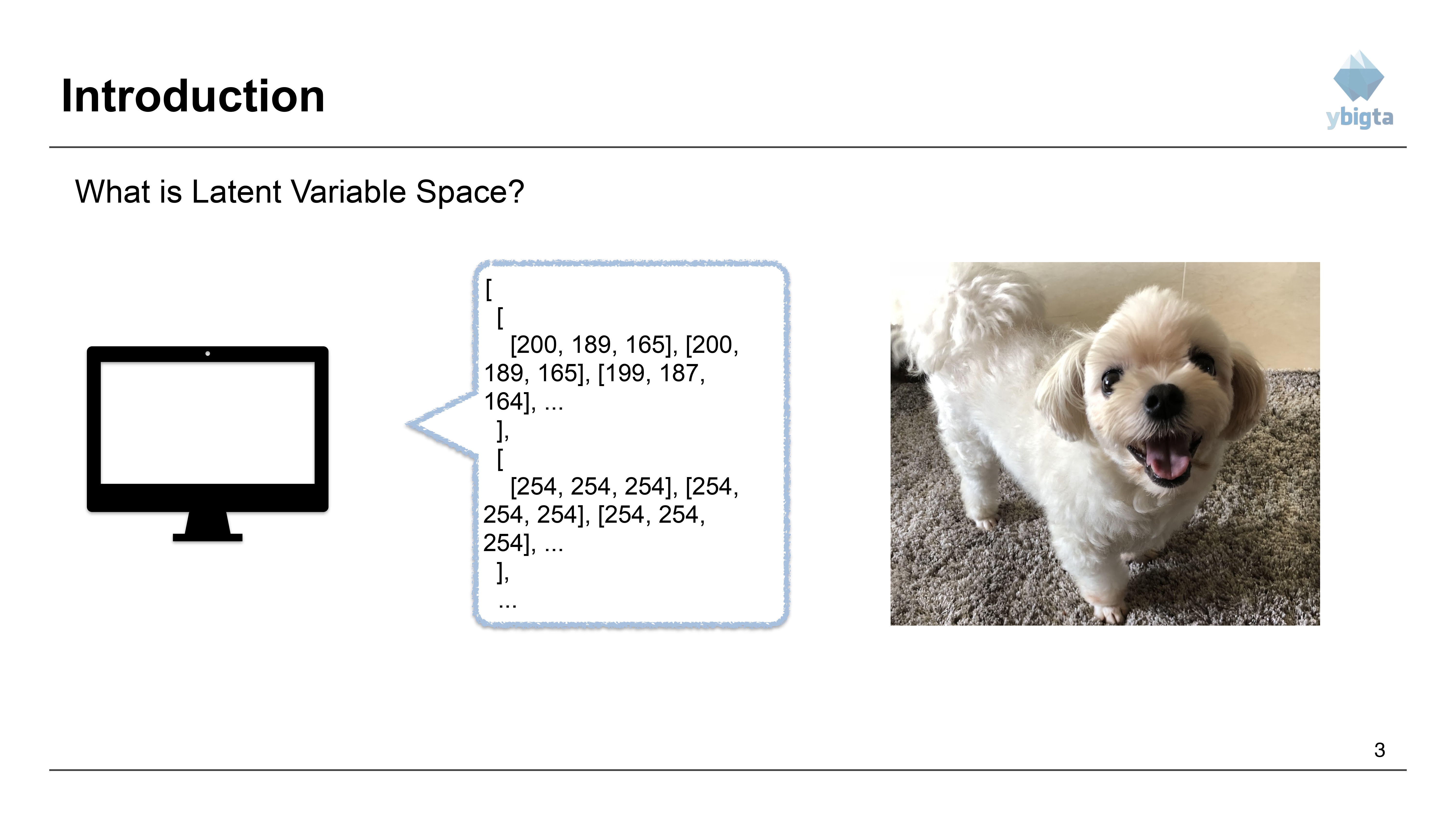
Slide 3: Computer Representation
- Computer view: The image is represented as a large tensor of pixel values (e.g., RGB arrays like
[200, 189, 165]...).
Slide 4: Latent Variable Space (1)
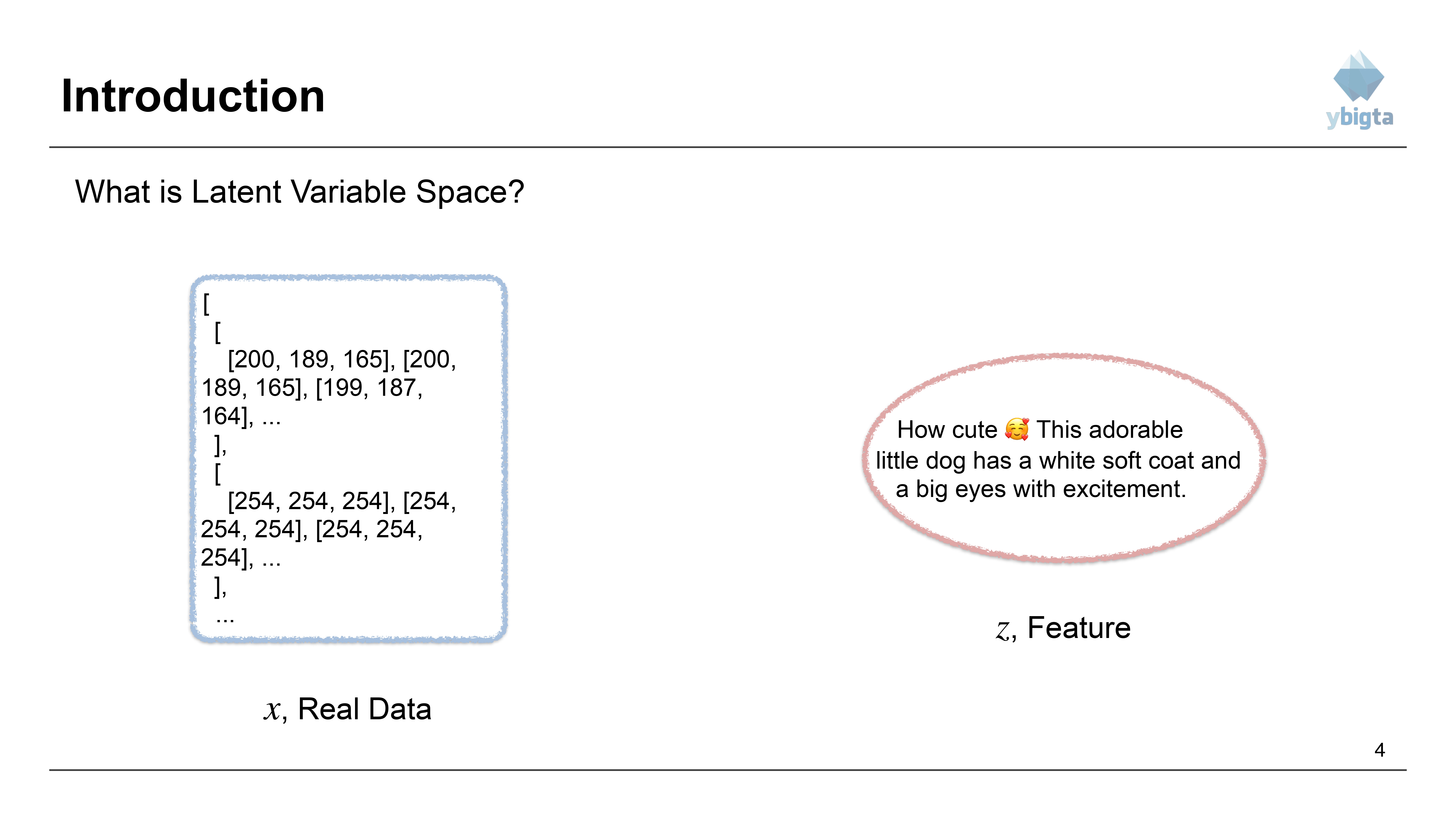
- Concept: Introduction to Latent Variable Space.
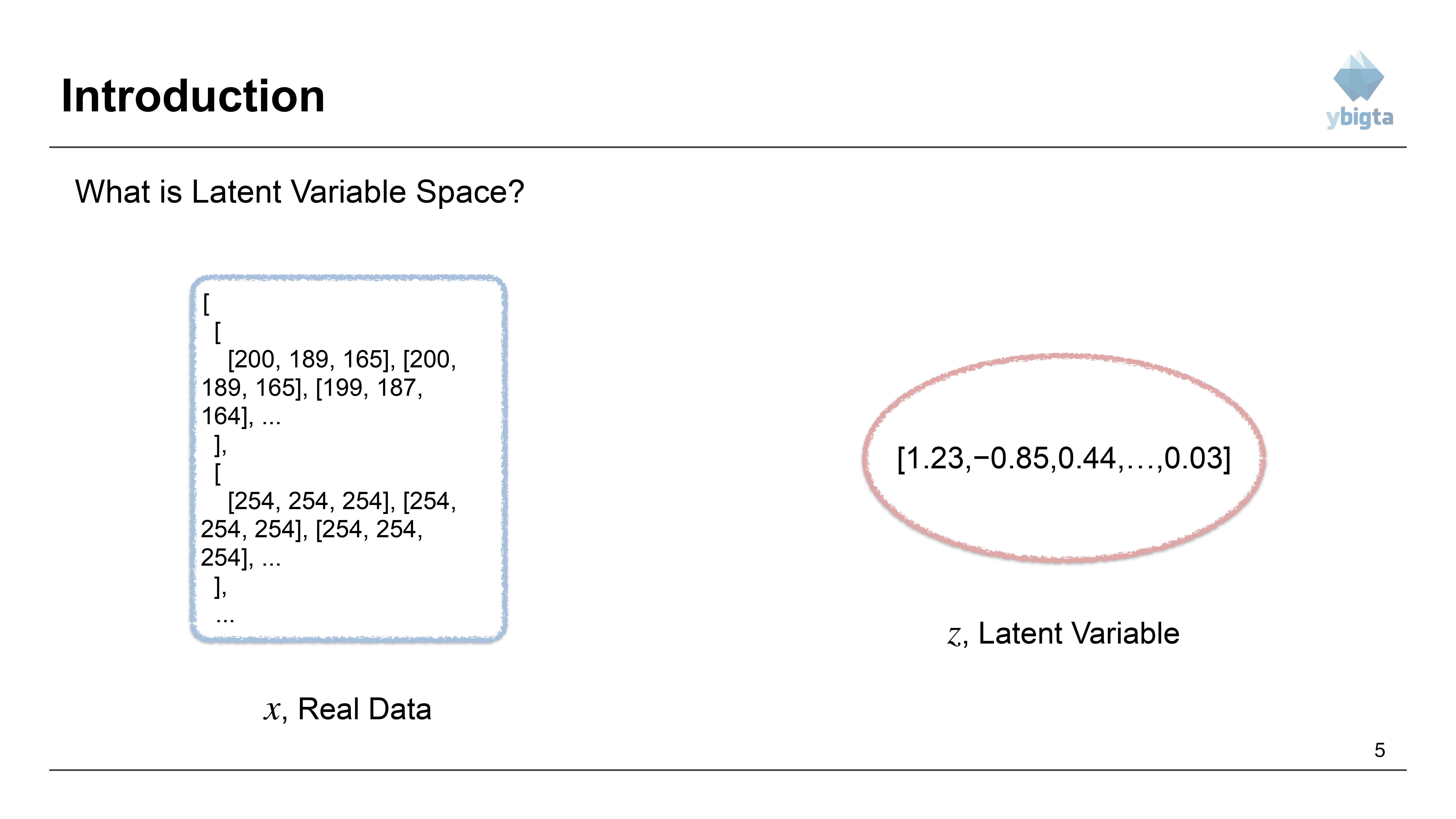
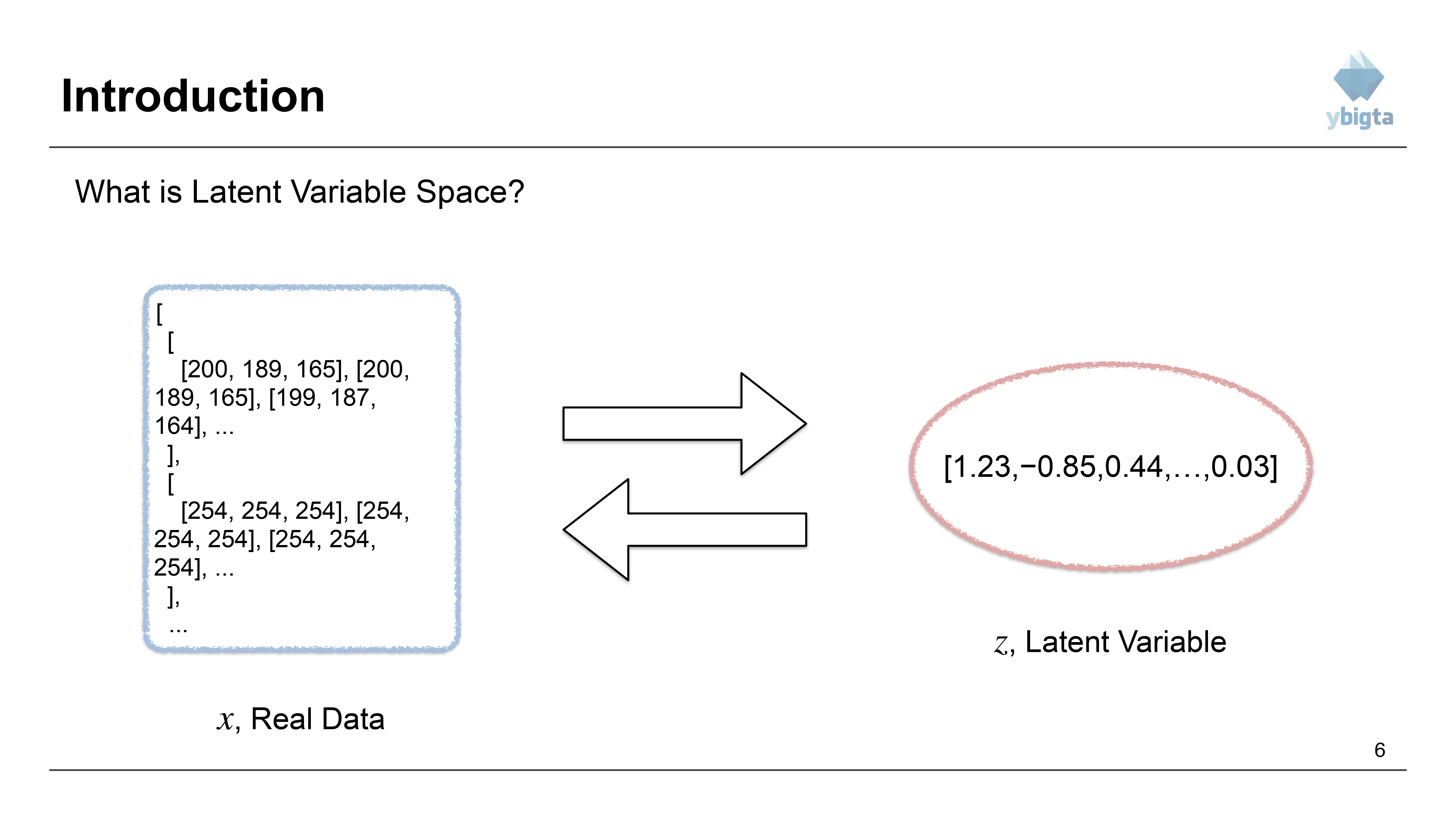
- We want to map the high-dimensional raw pixel data (Real Data, $x$) to a more meaningful, compressed representation.
- The descriptive features (“How cute”, “white soft coat”) represent the abstract information we want to capture.
Slide 5: Latent Variable Space (2)
- $x$ (Real Data): High-dimensional pixel array.
- Latent Variable: A compressed vector (e.g.,
[1.23, -0.85, 0.44, ..., 0.03]) that encodes the semantic features of the data.
Slide 6: Latent Variable Space (3)
- Visualizing the relationship: The raw data array corresponds to the latent vector.
Slide 7: Mapping Semantics
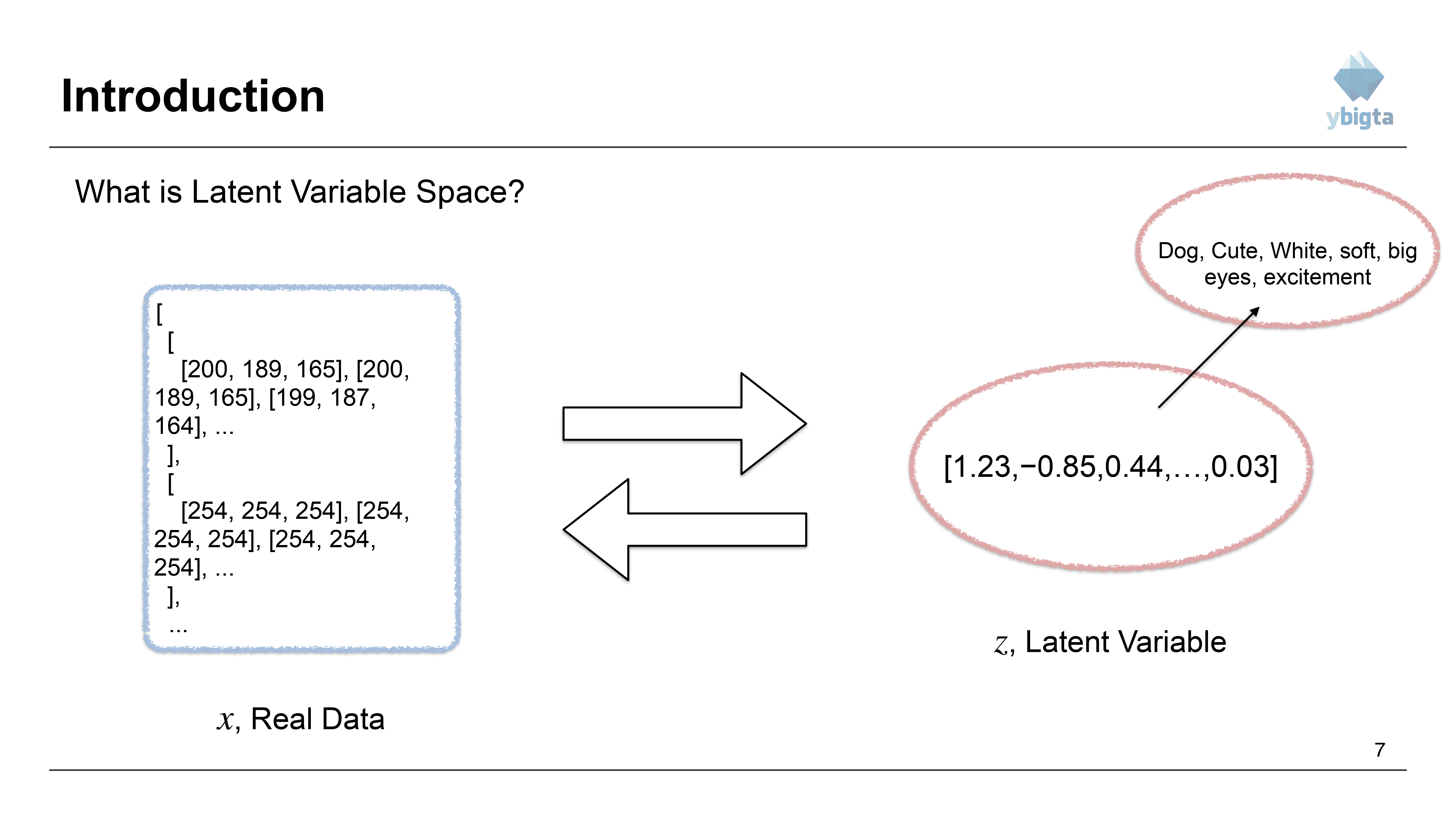
- Latent Variable: Represents features like “Dog”, “Cute”, “White”, “soft”, “big eyes”, “excitement”.
- These abstract concepts are encoded into the numeric vector $z$.
Slide 8: The Generative Goal
- Goal: To establish a two-way mapping.
- $x \to z$: Encoding the image into latent features.
- $z \to x$: Generating the image from latent features.
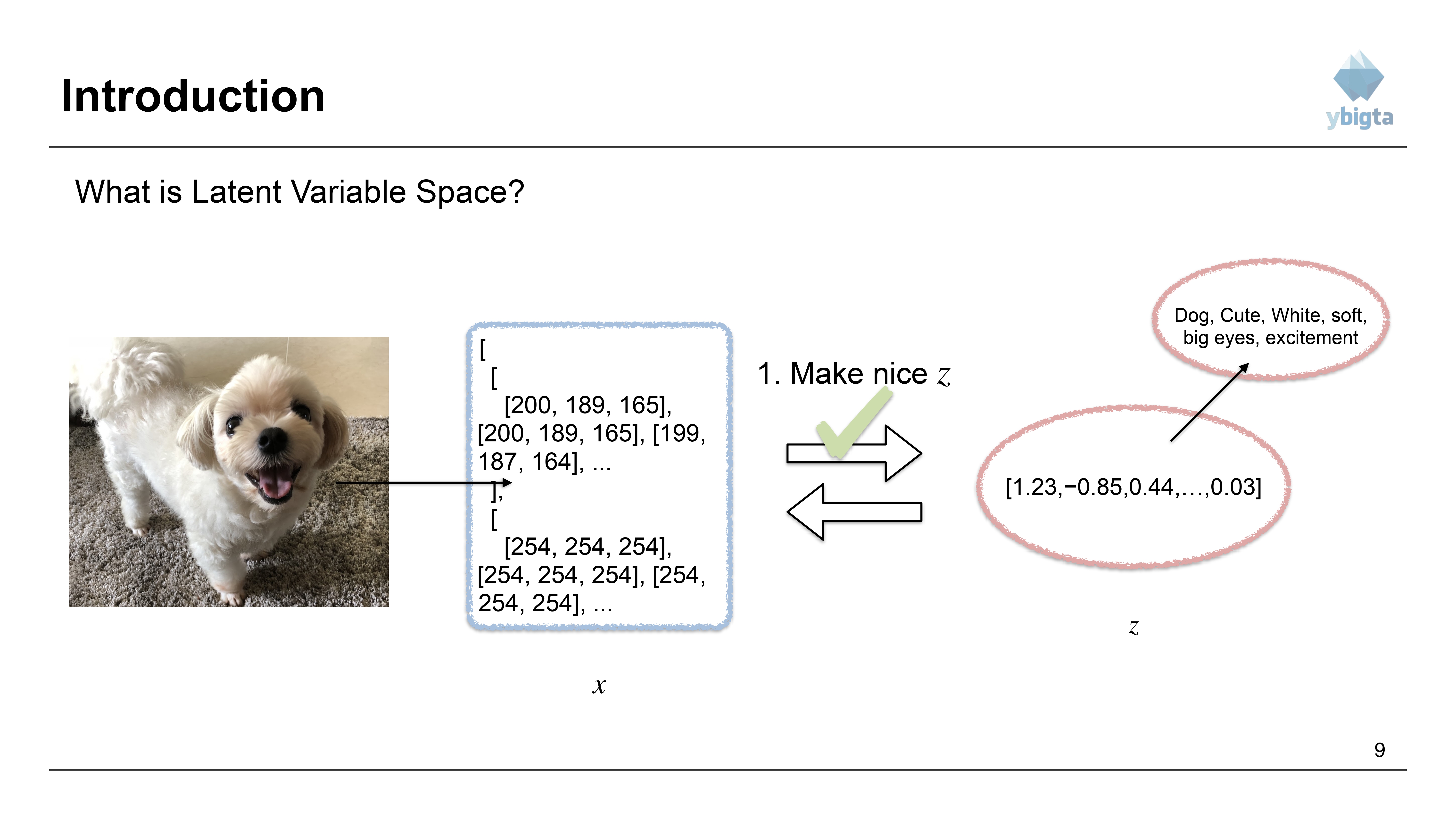
Slide 9: The Process
- Make nice $z$: Generate a meaningful latent vector from semantic descriptions or distributions.
- Reconstruct image: Use $z$ to create $x$.
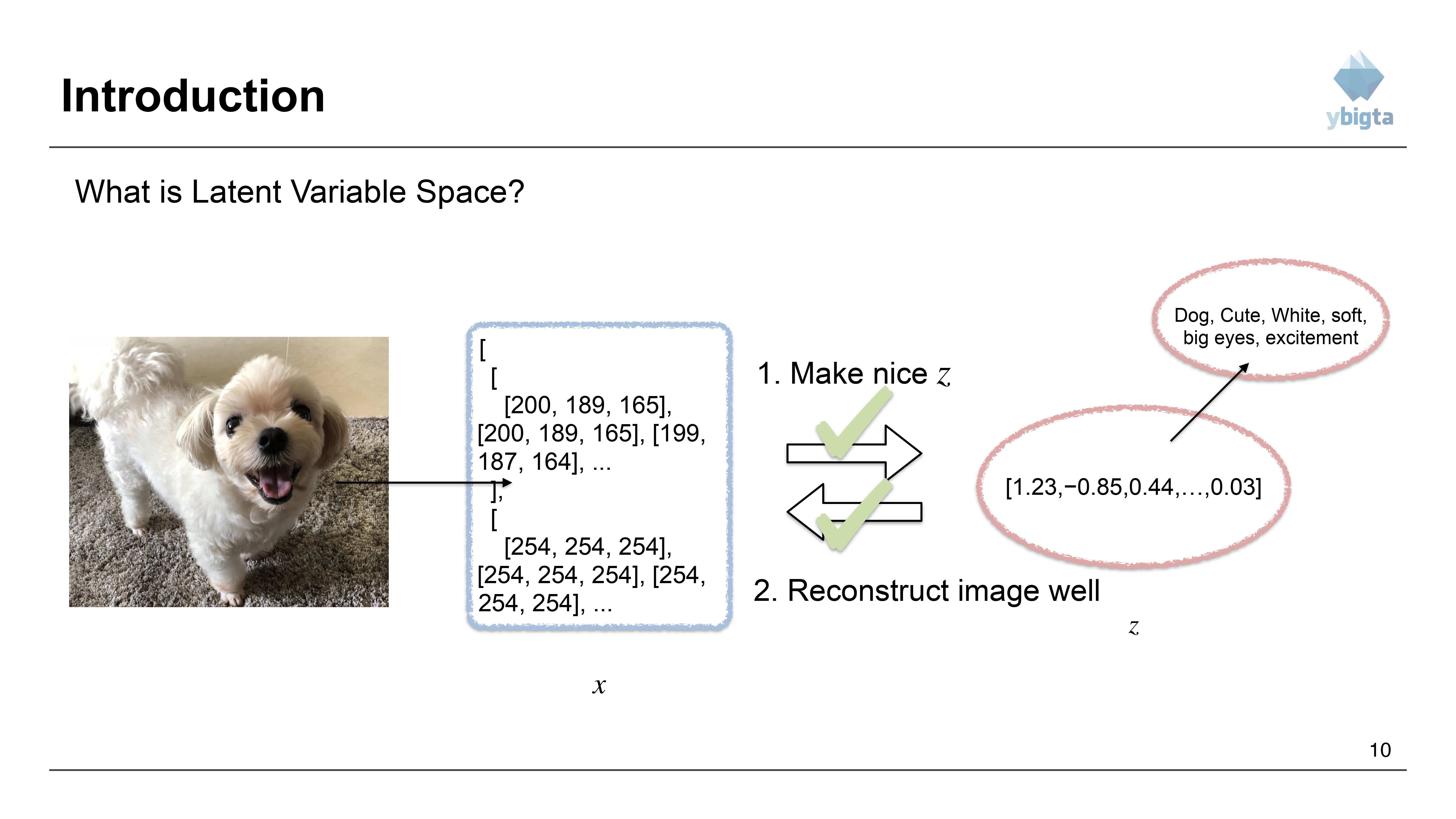
Slide 10: Requirements for a Good Model
- Make nice $z$: The latent space should be well-structured (e.g., following a standard normal distribution).
- Reconstruct image well: The generated image should look like the real data.
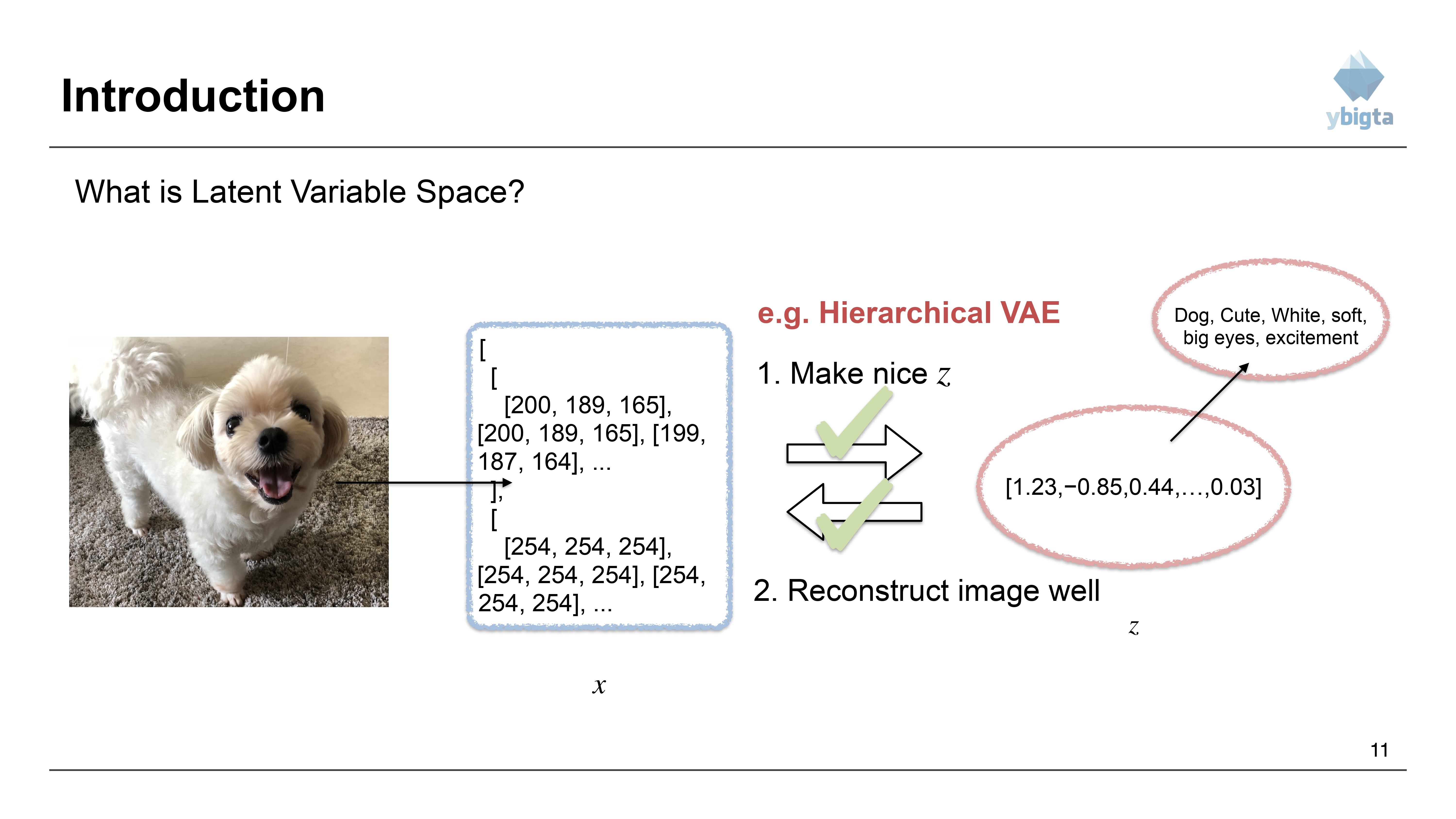
Slide 11: Example - Hierarchical VAE
- Hierarchical VAE: An extension of standard VAEs.
- Uses multiple layers of latent variables ($z_1, z_2, …$) to capture features at different levels of abstraction.
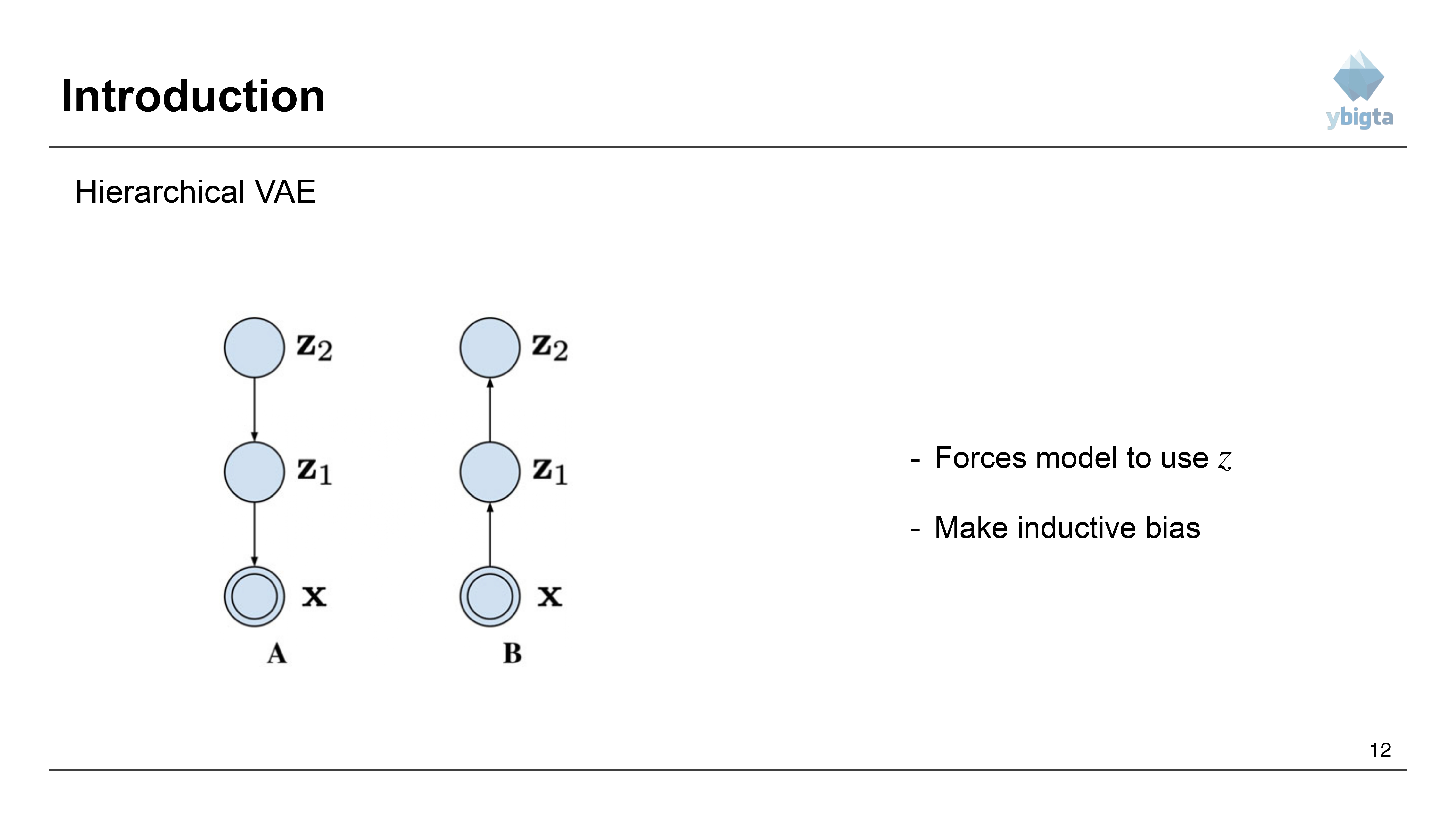
Slide 12: Hierarchical VAE Structure
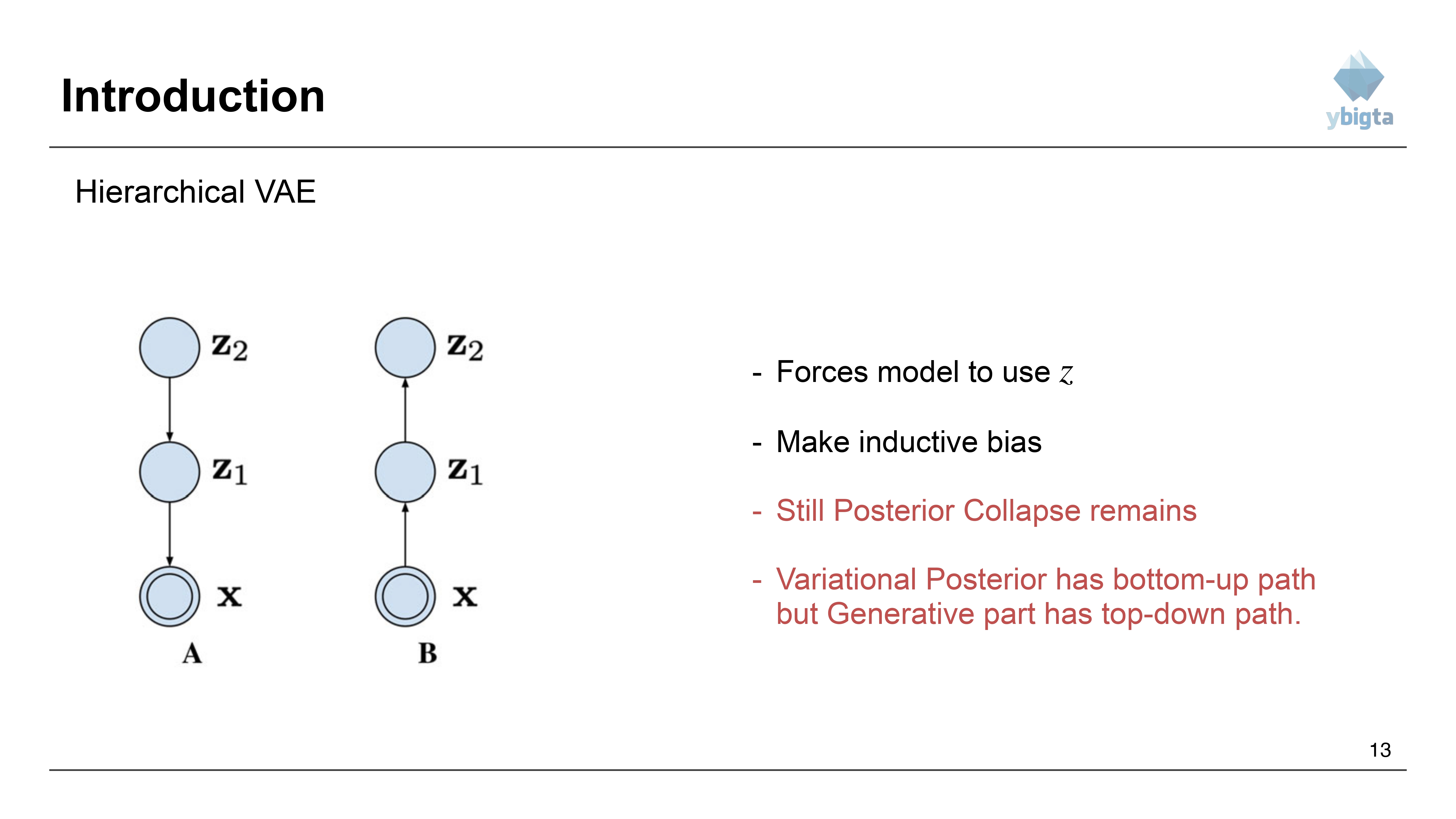
- Structure:
- A (Generative/Top-down): $z_2 \to z_1 \to x$.
- B (Inference/Bottom-up): $x \to z_1 \to z_2$.
- Objective: Forces the model to use $z$ to create an Inductive Bias.
Slide 13: The Problem - Posterior Collapse
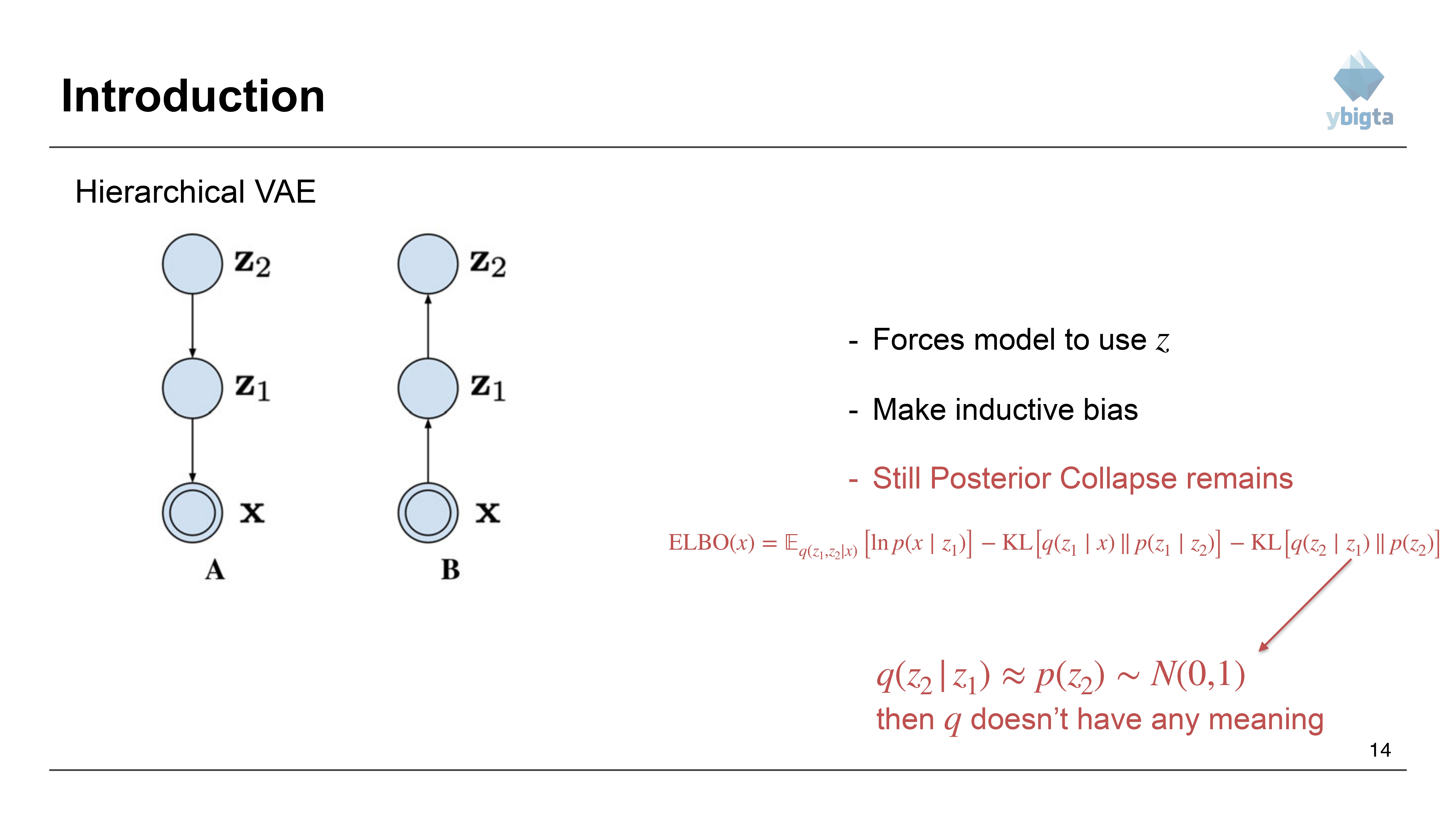
- Even with hierarchy, Posterior Collapse remains a problem.
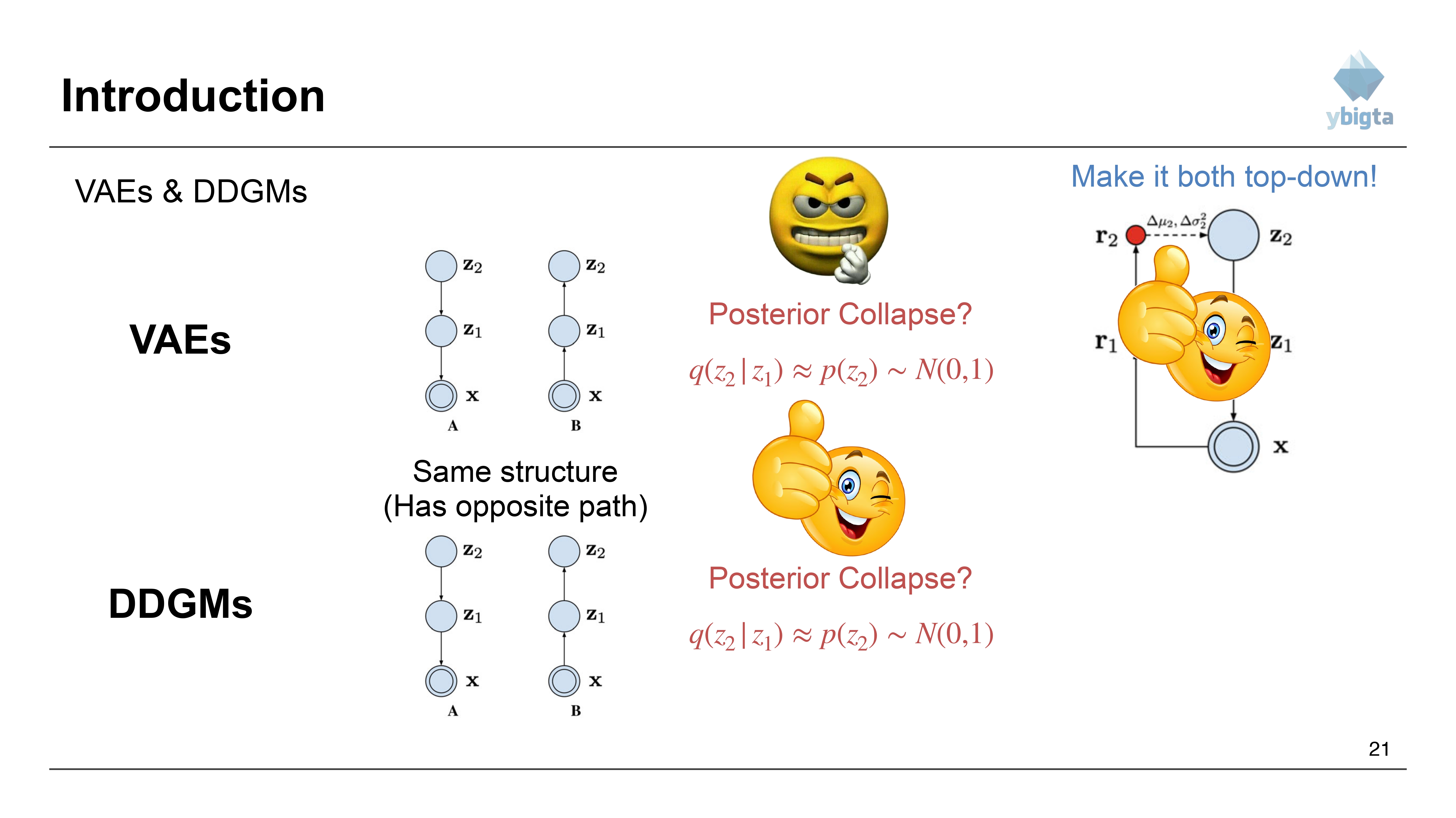
- Issue: The variational posterior has a bottom-up path, but the generative part has a top-down path.
- Sometimes the model ignores the latent code $z$ and relies solely on the powerful decoder (autoregressive part), making $z$ meaningless.
Slide 14: Analyzing Posterior Collapse
- ELBO Equation: $$ELBO(x) = E_{q(z_1:z_2|x)}[\ln p(x|z_1)] - KL[q(z_1|x)||p(z_1|z_2)] - KL[q(z_2|z_1)||p(z_2)]$$
- Collapse condition: If $q(z_2|z_1) \approx p(z_2) \sim \mathcal{N}(0,1)$, then $q$ doesn’t encode any meaningful information about the data.
Slide 15: Hierarchical VAE (Top-down Inference)
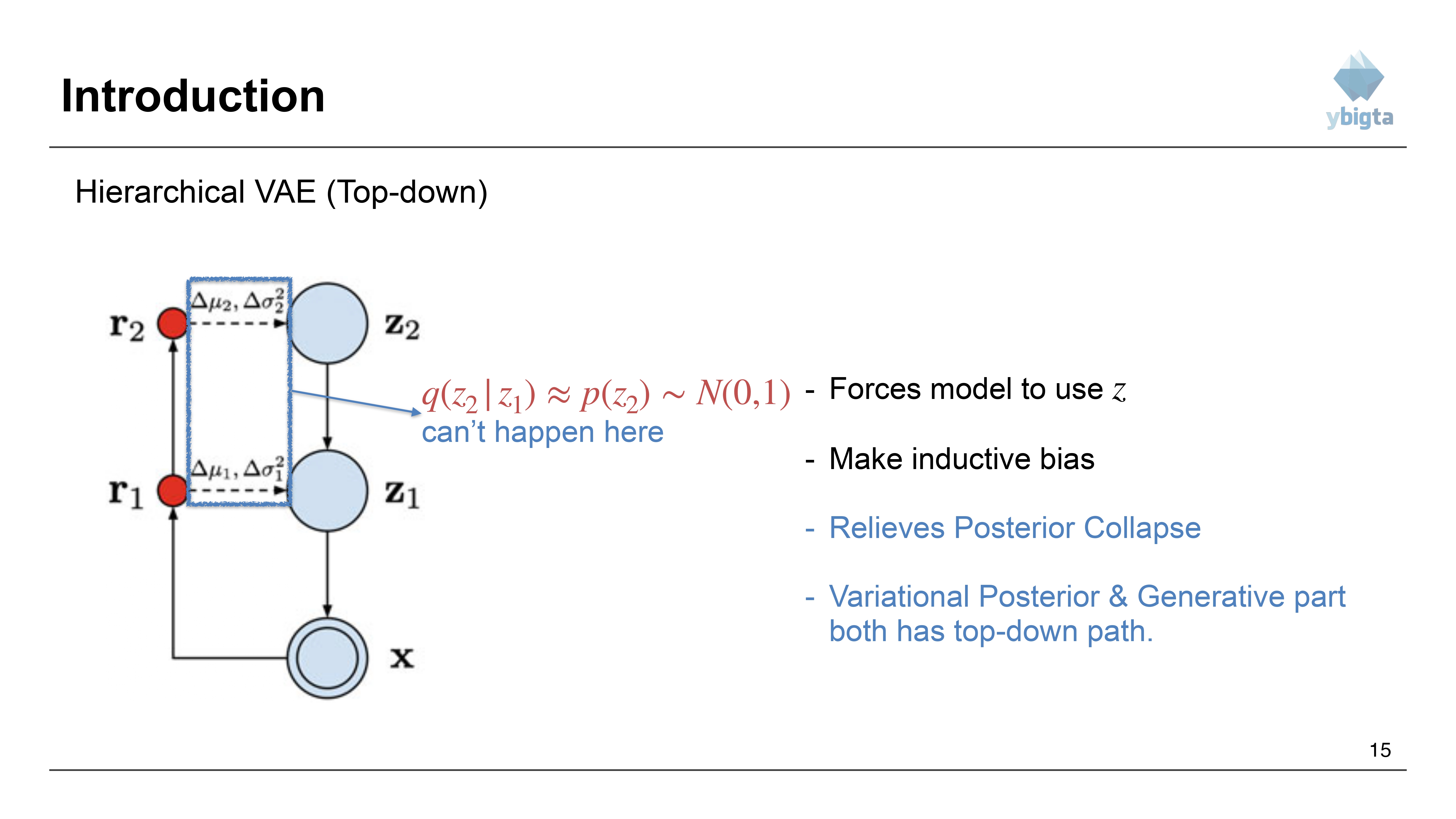
- Solution attempt: Make the variational posterior top-down as well.
- Mechanism: Use residual connections ($r_1, r_2$) and delta parameters ($\Delta\mu, \Delta\sigma^2$) to guide the generation.
- Benefit:
- Forces the model to use $z$.
- Creates stronger inductive bias.
- Relieves Posterior Collapse because both Variational Posterior & Generative parts have a top-down path.
- Note: $q(z_2|z_1) \approx p(z_2)$ cannot happen easily here.
Slide 16: Introduction to Diffusion Based Deep Generative Models
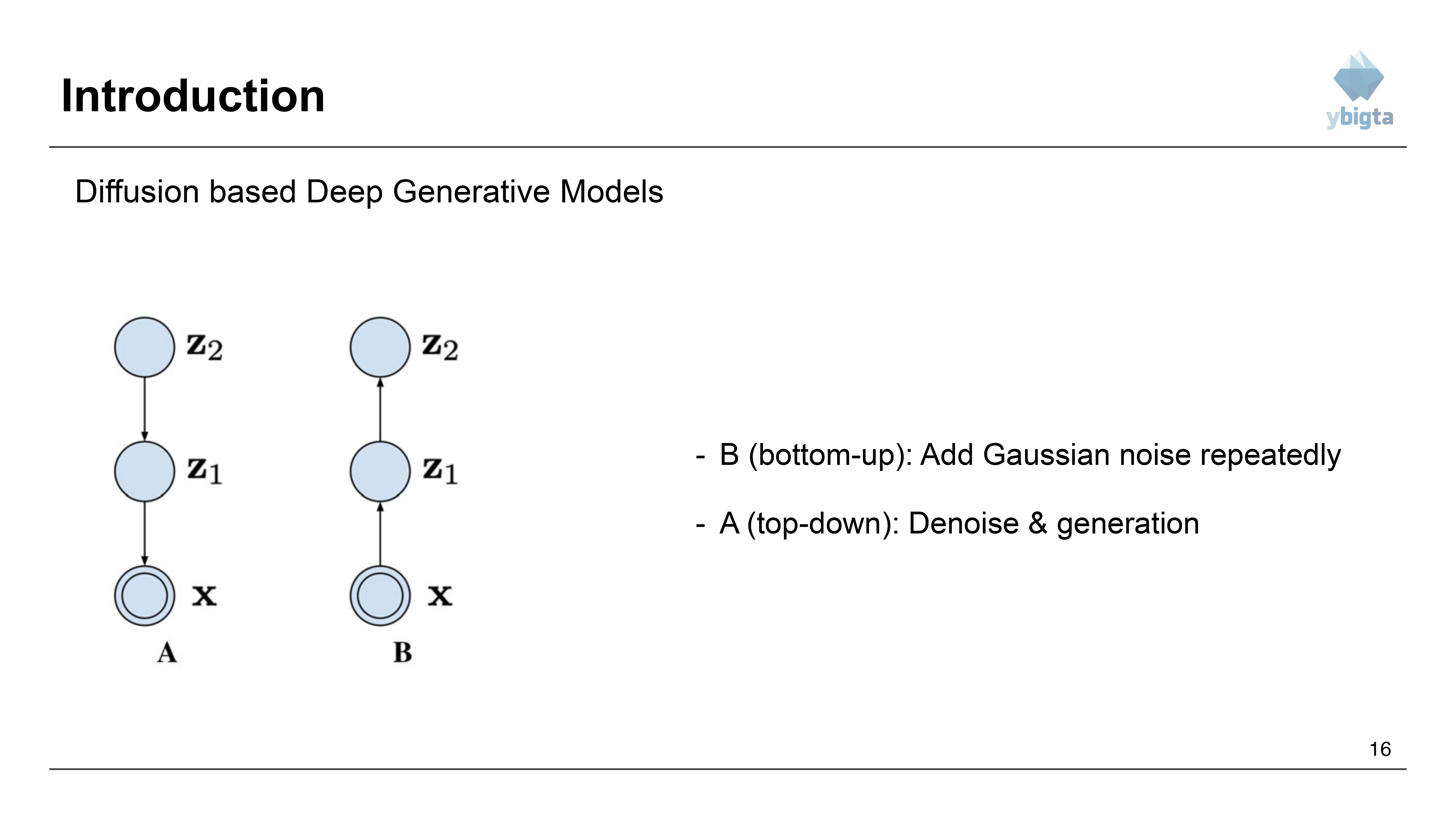
- Comparing the structures.
- Diffusion Models:
- B (Bottom-up): Add Gaussian noise repeatedly.
- A (Top-down): Denoise & generation.
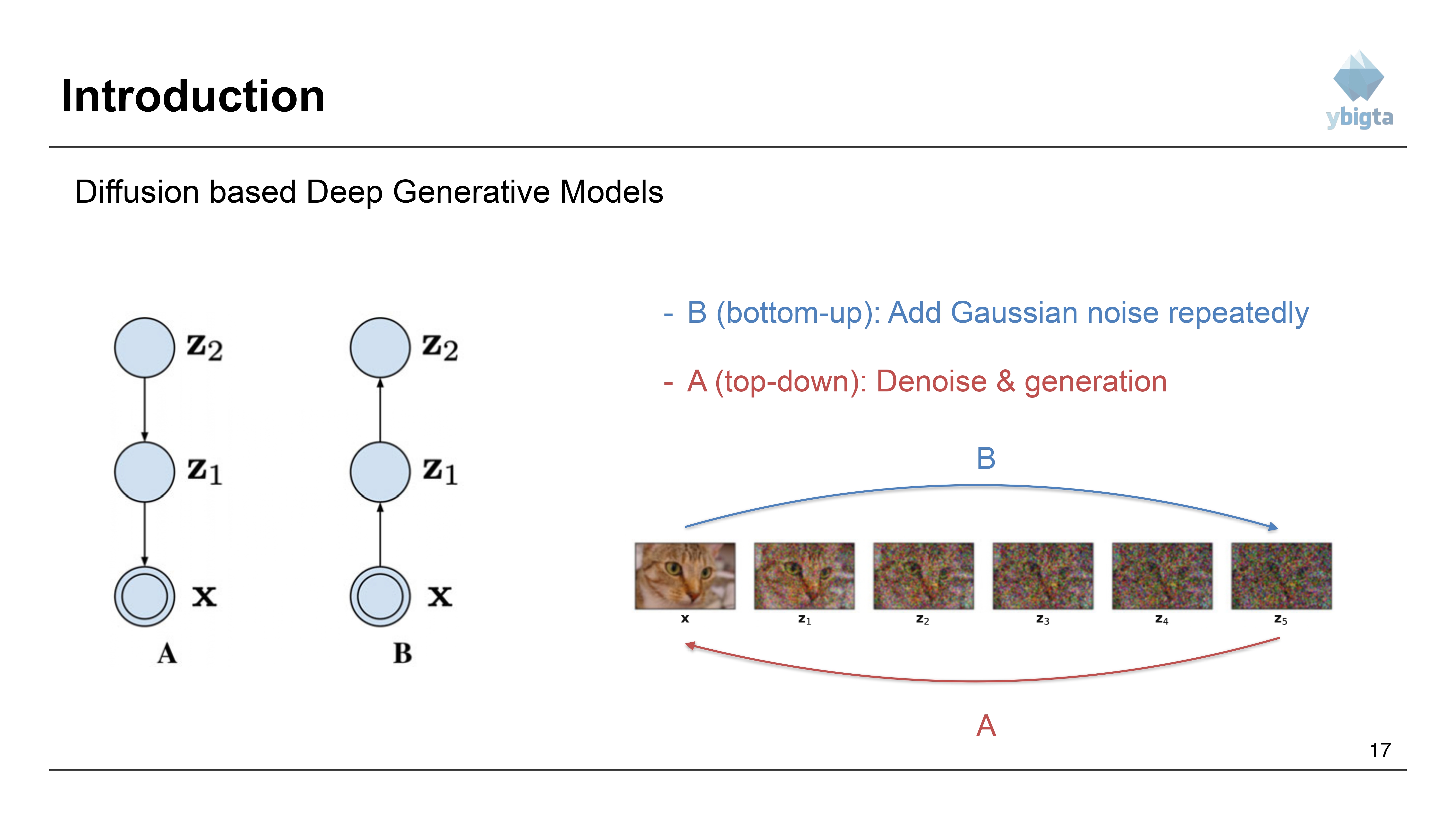
Slide 17: Diffusion Process Visualization
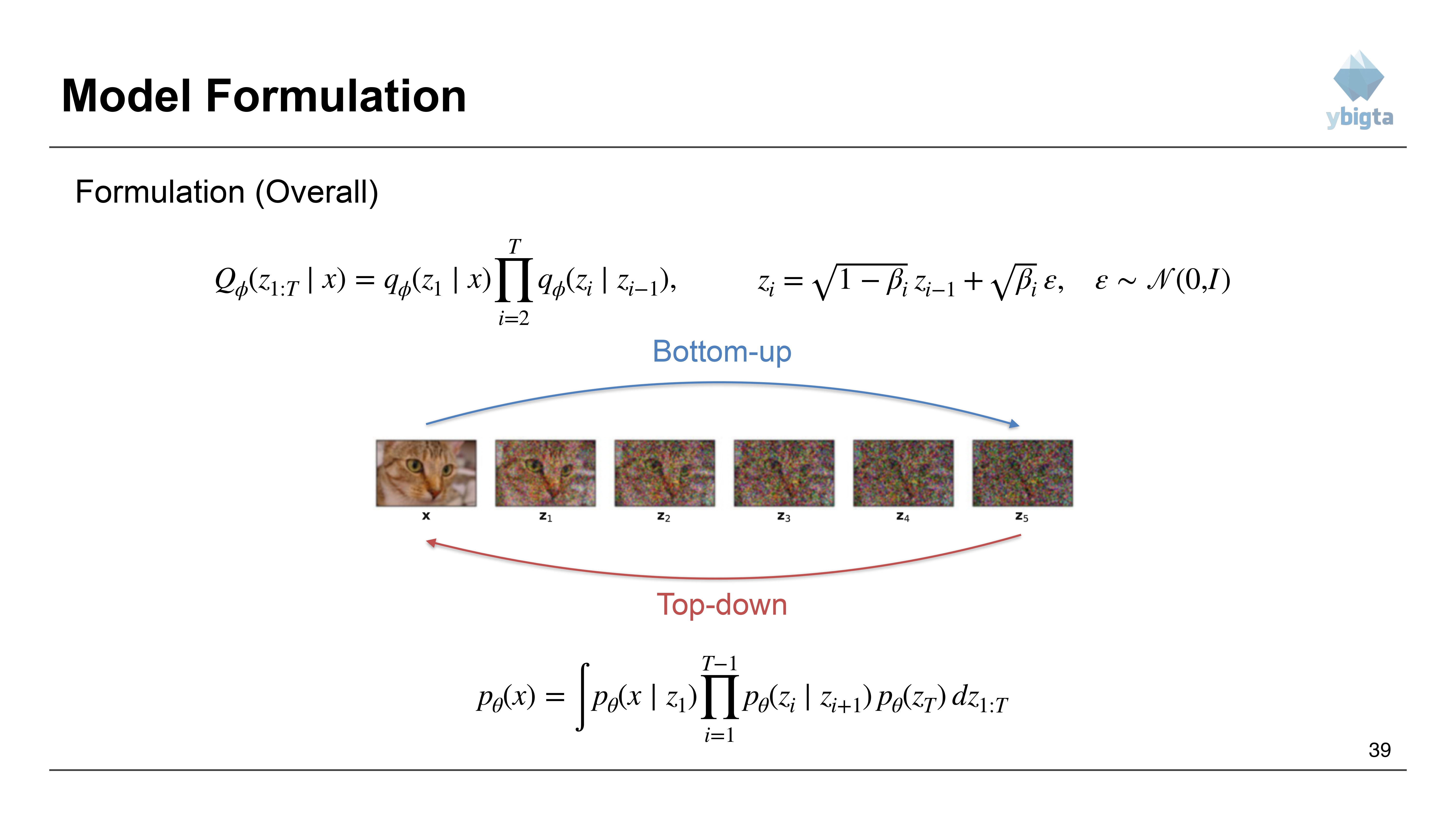
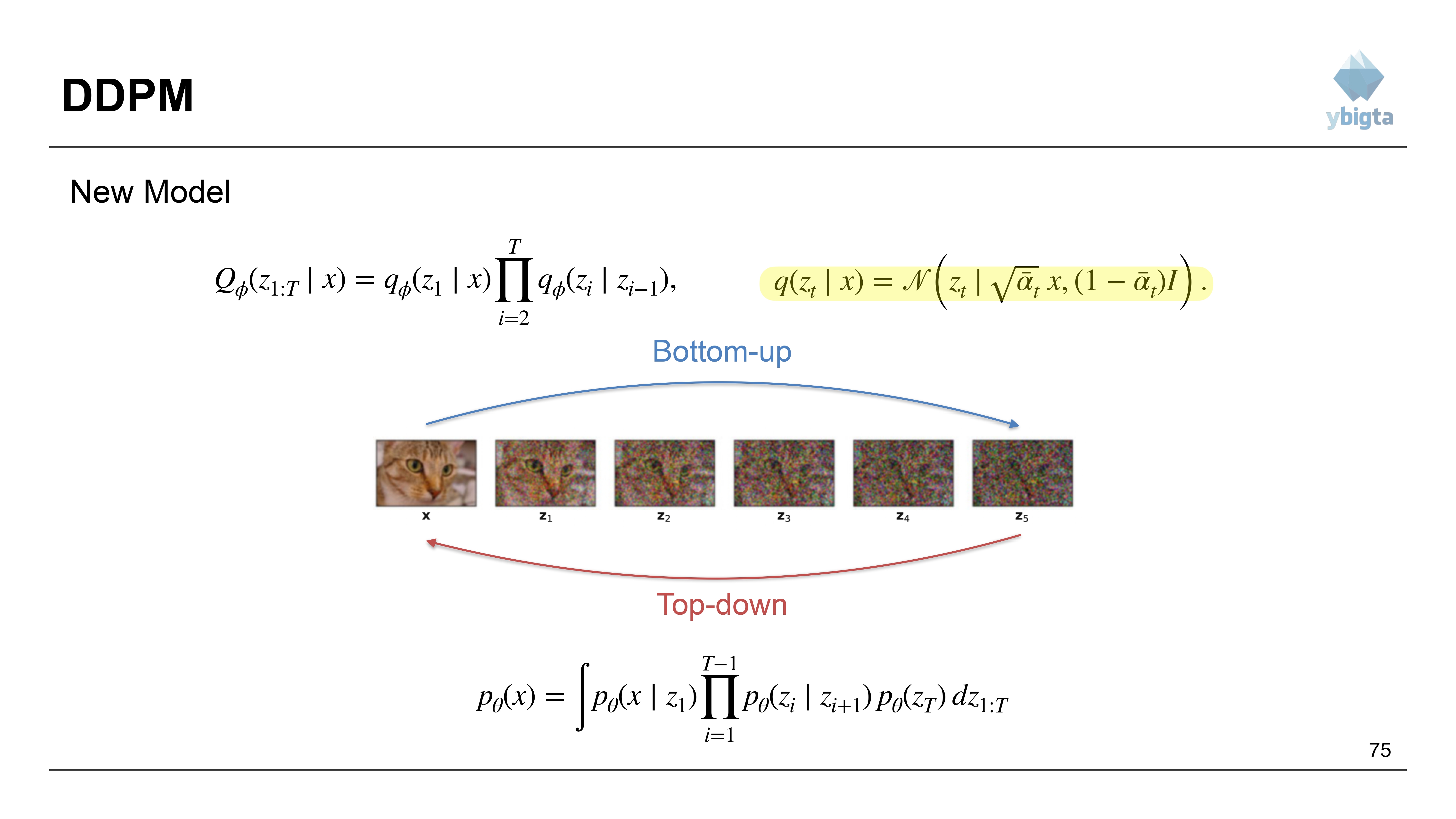
- Forward (B): Start with image $x$ -> add noise -> $z_1$ -> … -> $z_5$ (pure noise).
- Reverse (A): Start with noise $z_5$ -> denoise -> … -> generate $x$.
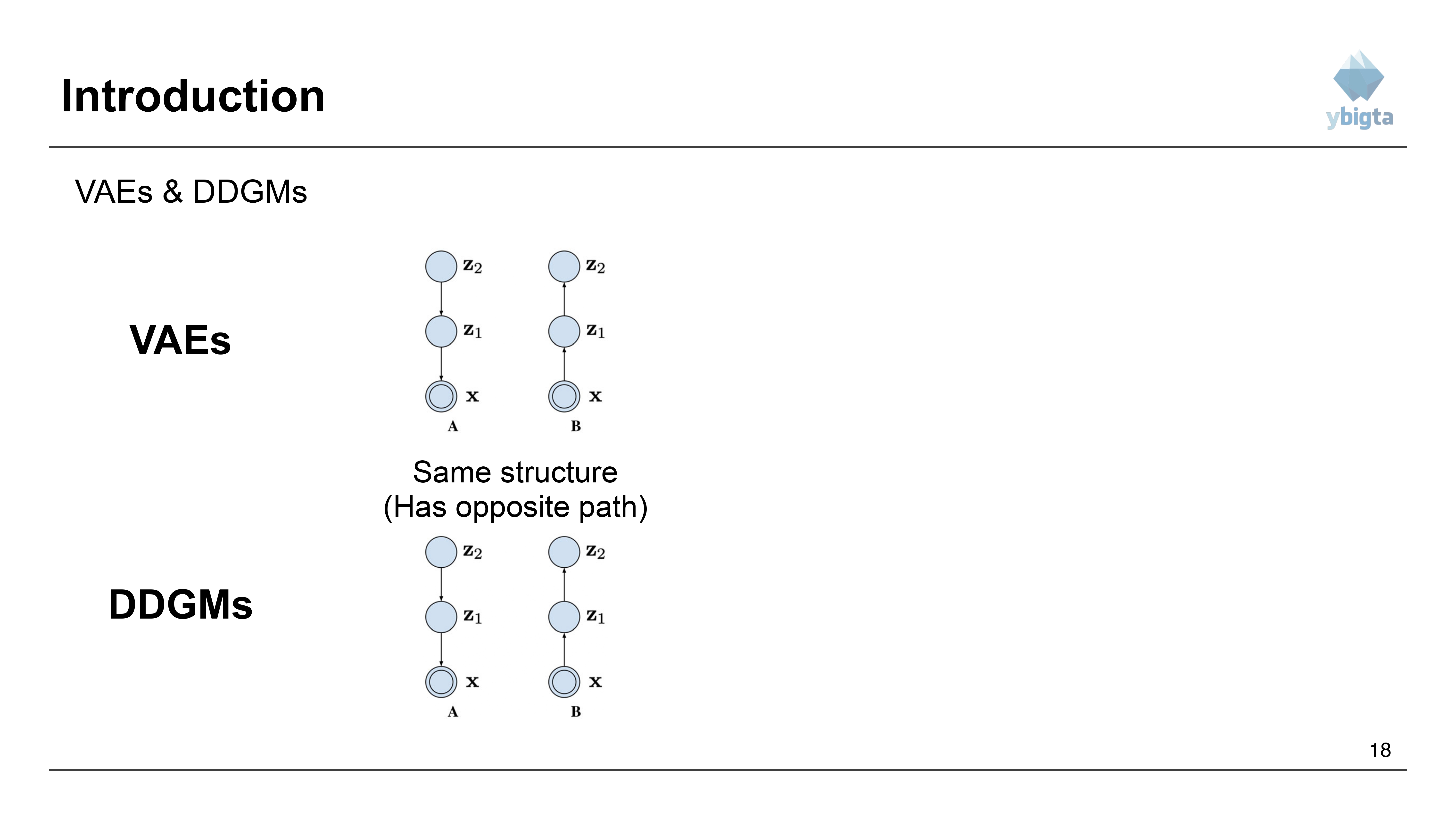
Slide 18: VAEs vs. DDGMs (Structural Comparison)
- VAEs:
- A (Generative): Top-down ($z_2 \to z_1 \to x$).
- B (Inference): Bottom-up ($x \to z_1 \to z_2$).
- Structure has opposite paths.
- DDGMs (Diffusion):
- A (Generative): Top-down ($z_2 \to z_1 \to x$).
- B (Inference): Bottom-up ($x \to z_1 \to z_2$).
- Same structure visually, but distinct operational paths.
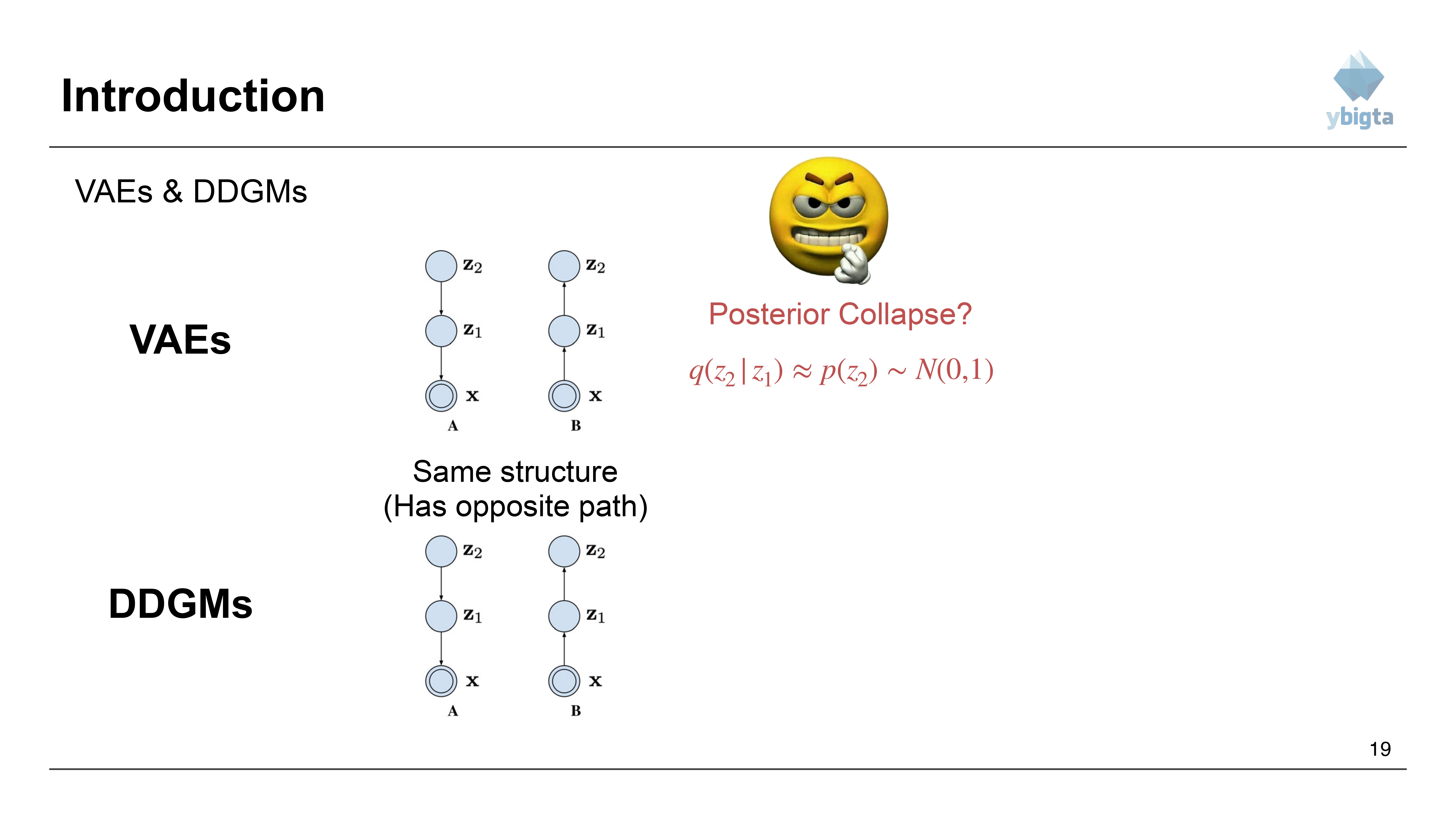
Slide 19: Addressing Posterior Collapse in DDGMs
- Question: Does Posterior Collapse happen in DDGMs?
- VAE: Often suffers from $q(z_2|z_1) \approx p(z_2) \sim \mathcal{N}(0,1)$.
- DDGM: The structure is similar (opposite paths), so we need to check.
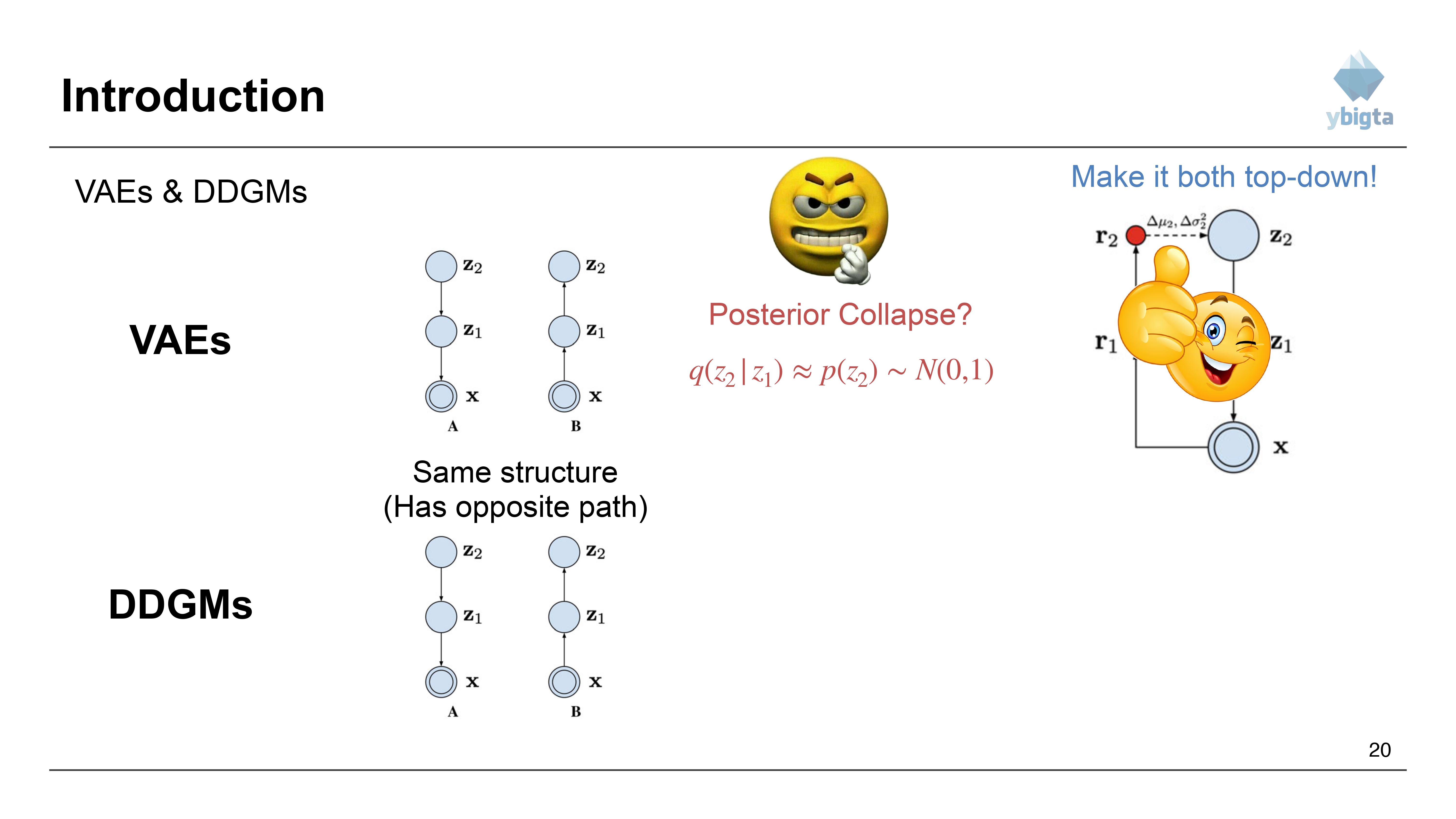
Slide 20: Top-Down Fix in VAEs
- Recall slide 15: VAEs fixed collapse by making both paths top-down using ResNet-like connections.
- Does Diffusion do this?
Slide 21: Diffusion’s Approach
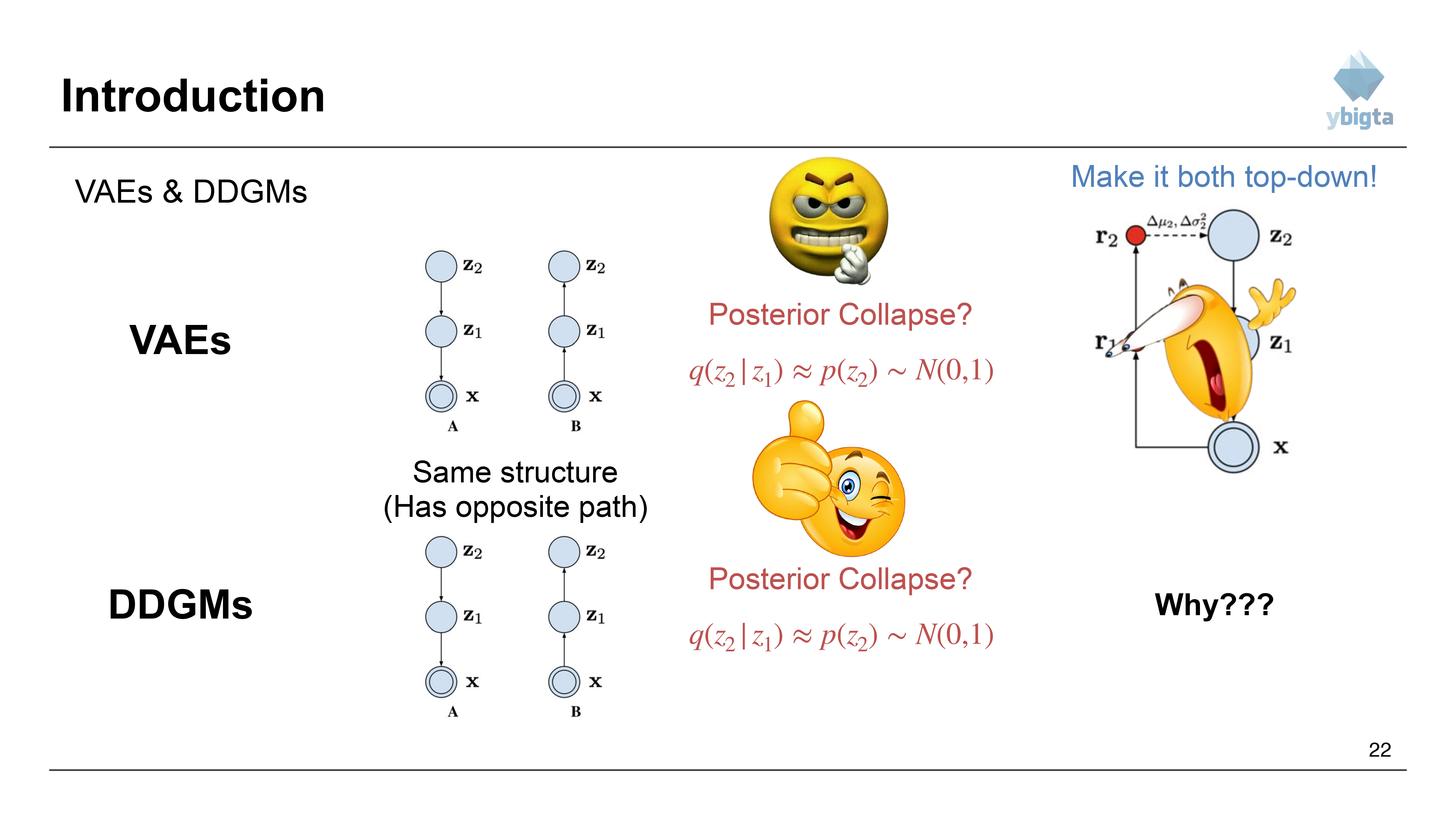
- Diffusion models have the standard opposite path structure (Forward vs Reverse).
- Does Posterior Collapse remain?
- $q(z_2|z_1) \approx p(z_2) \sim \mathcal{N}(0,1)$?
- Answer: No.
Slide 22: Why No Posterior Collapse?
- In Diffusion, the forward process (Bottom-up B) is fixed to add noise. It forces the data to become Gaussian noise.
- It is not a learned parameter that can “collapse” to zero information; it is a fixed physical process.
Slide 23: Paper Introduction
- Paper: Deep Unsupervised Learning using Nonequilibrium Thermodynamics (ICML 2015).
- Authors: Jascha Sohl-Dickstein, Eric A. Weiss, Niru Maheswaranathan, Surya Ganguli.
Slide 24: Motivation - Nonequilibrium Thermodynamics
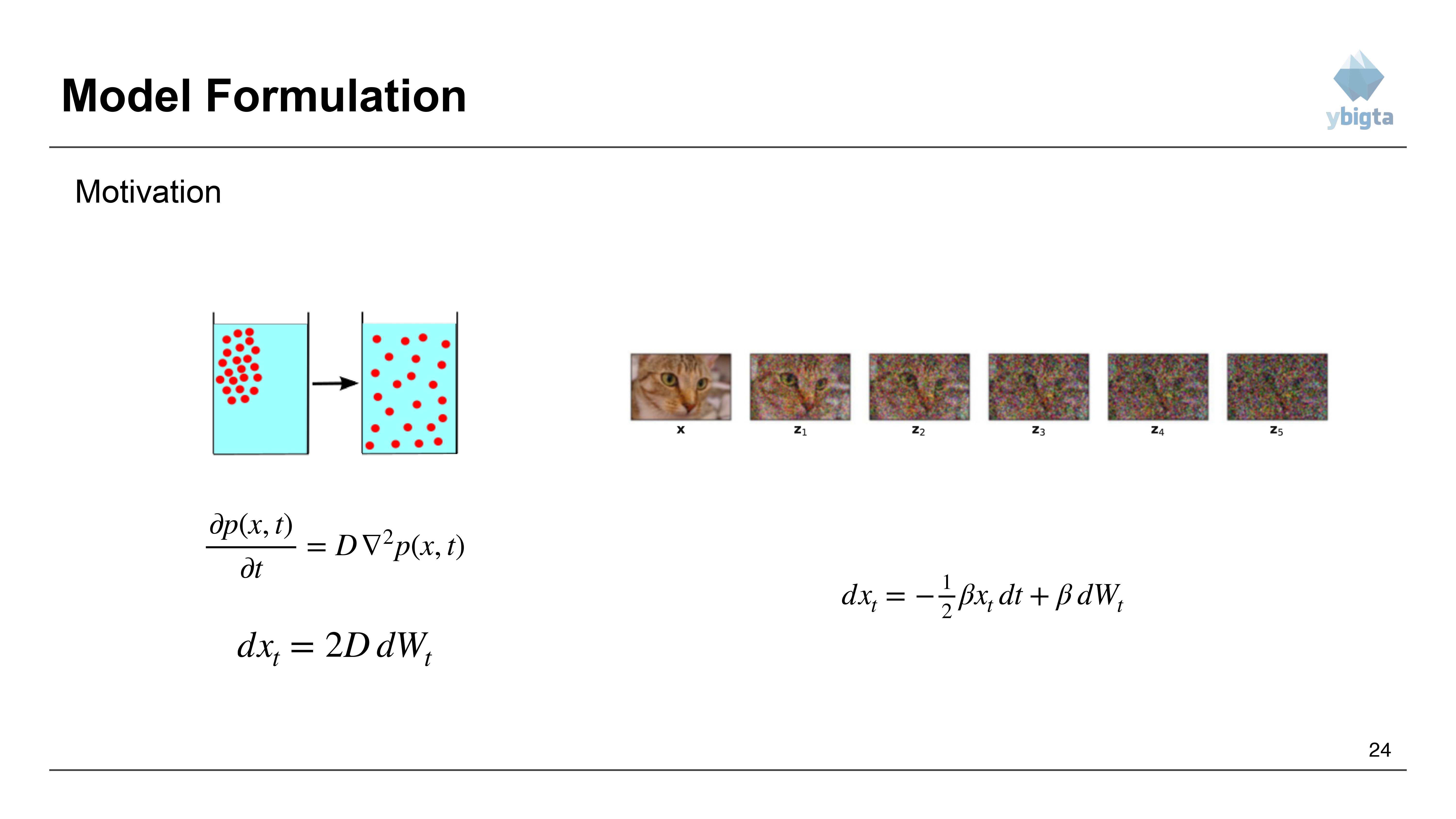
- Physical Analogy: A drop of ink diffusing in water.
- Equation: $\frac{\partial p(x,t)}{\partial t} = D\nabla^2 p(x,t)$
- Forward Process: $dx_t = -\frac{1}{2}\beta x_t dt + \beta dW_t$
- Organized structure (Ink drop) $\to$ Disorganized structure (Uniform distribution).
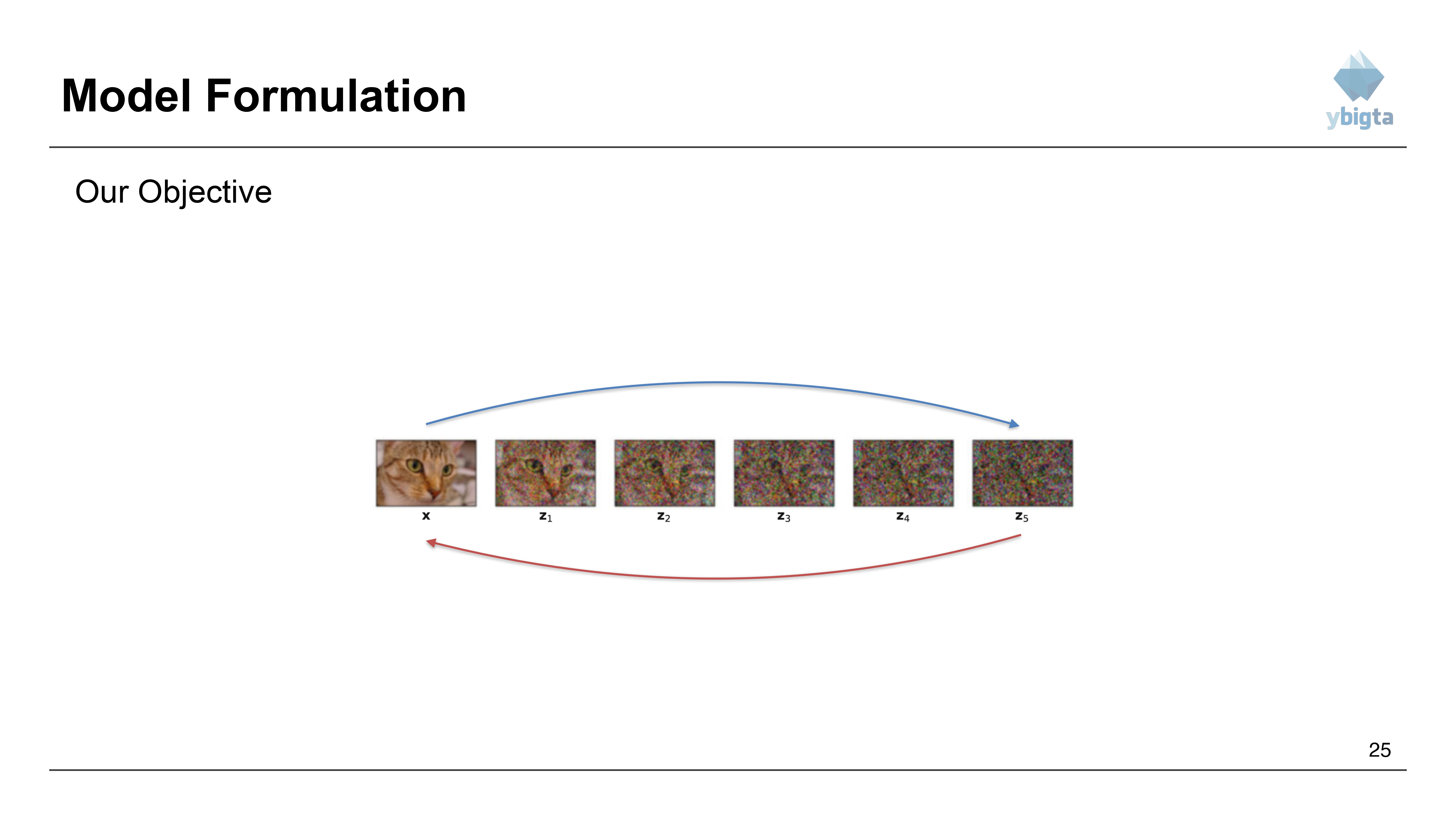
Slide 25: Our Objective
- Map the diffusion process to image generation.
- Sequence: $x \to z_1 \to z_2 \to z_3 \to z_4 \to z_5$ (Noise).
- We want to reverse this.
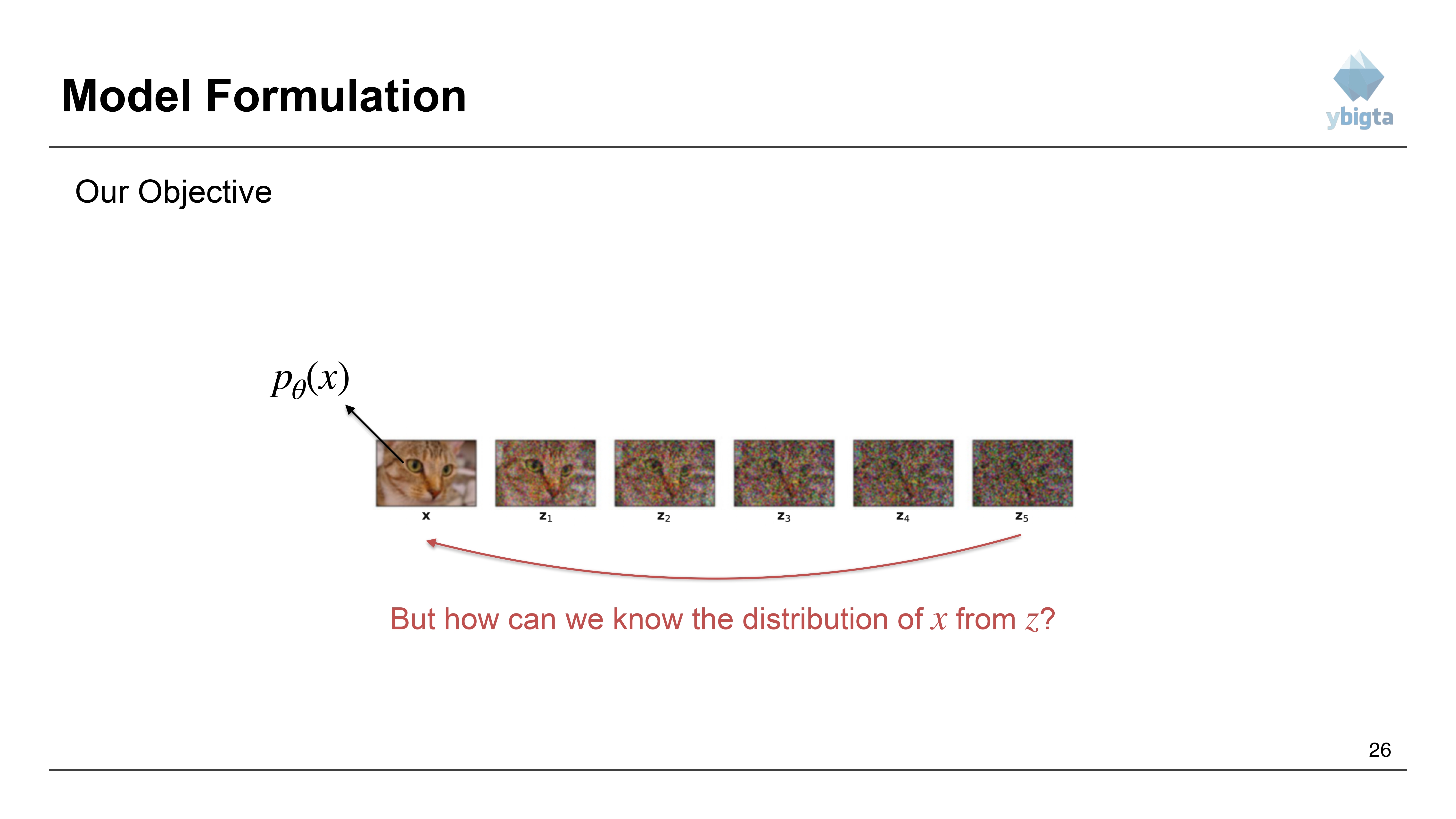
Slide 26: Defining the Target Distribution
- We want to learn the distribution $p_\theta(x)$ that generates the cat image.
- Problem: How can we know the distribution of $x$ from $z$?
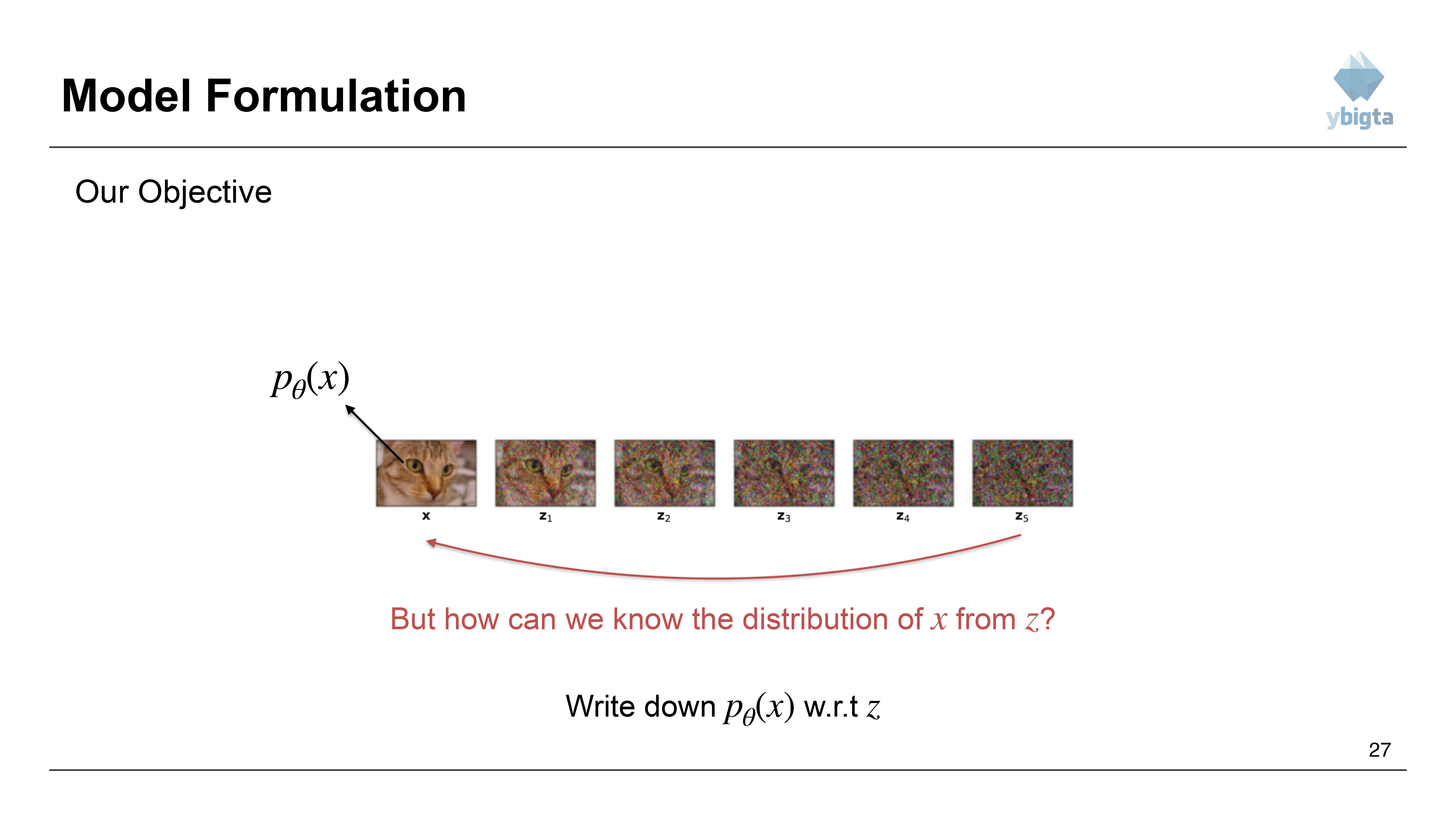
Slide 27: Formulation Strategy
- We need to write down $p_\theta(x)$ with respect to latent variables $z$.
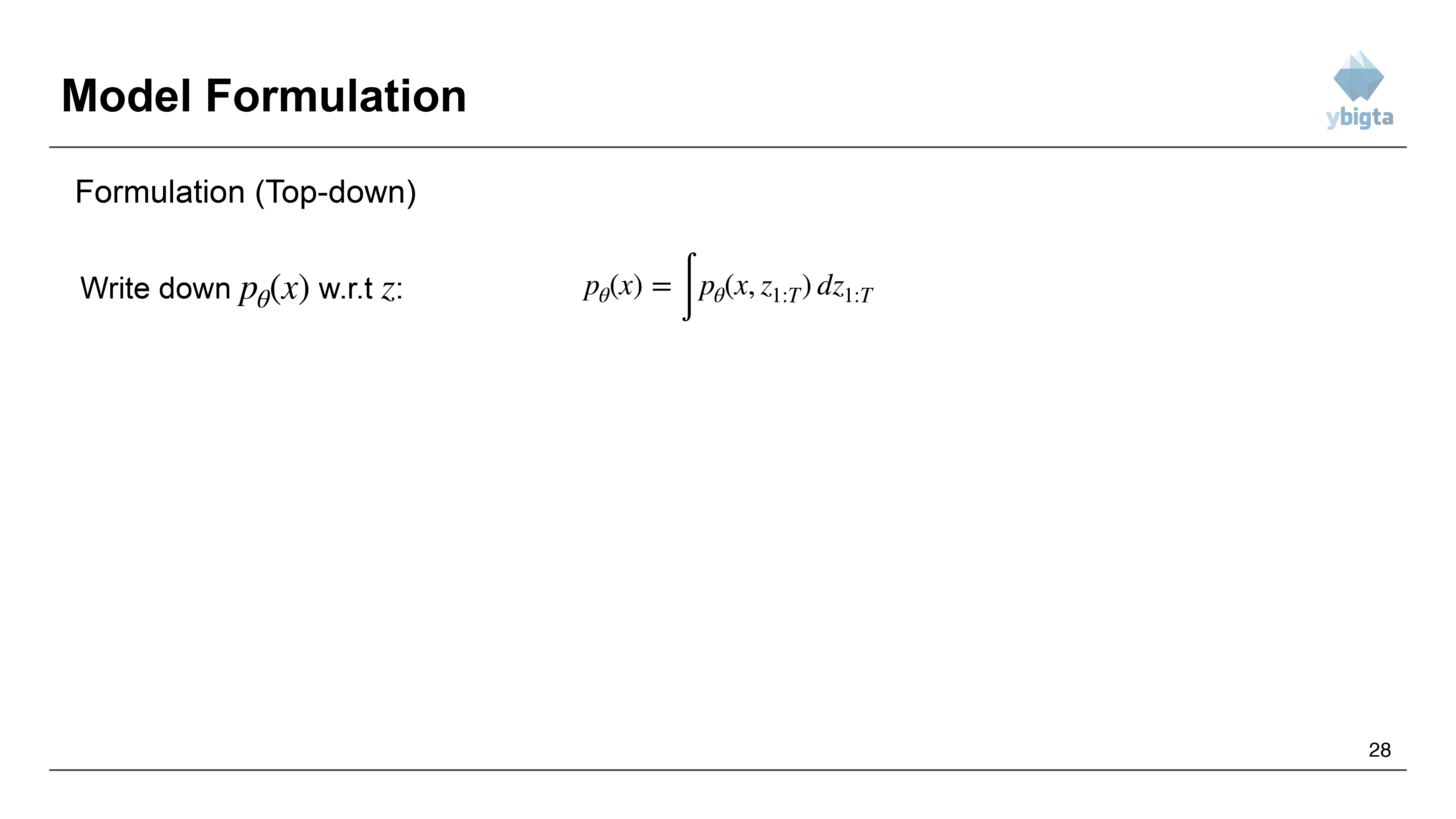
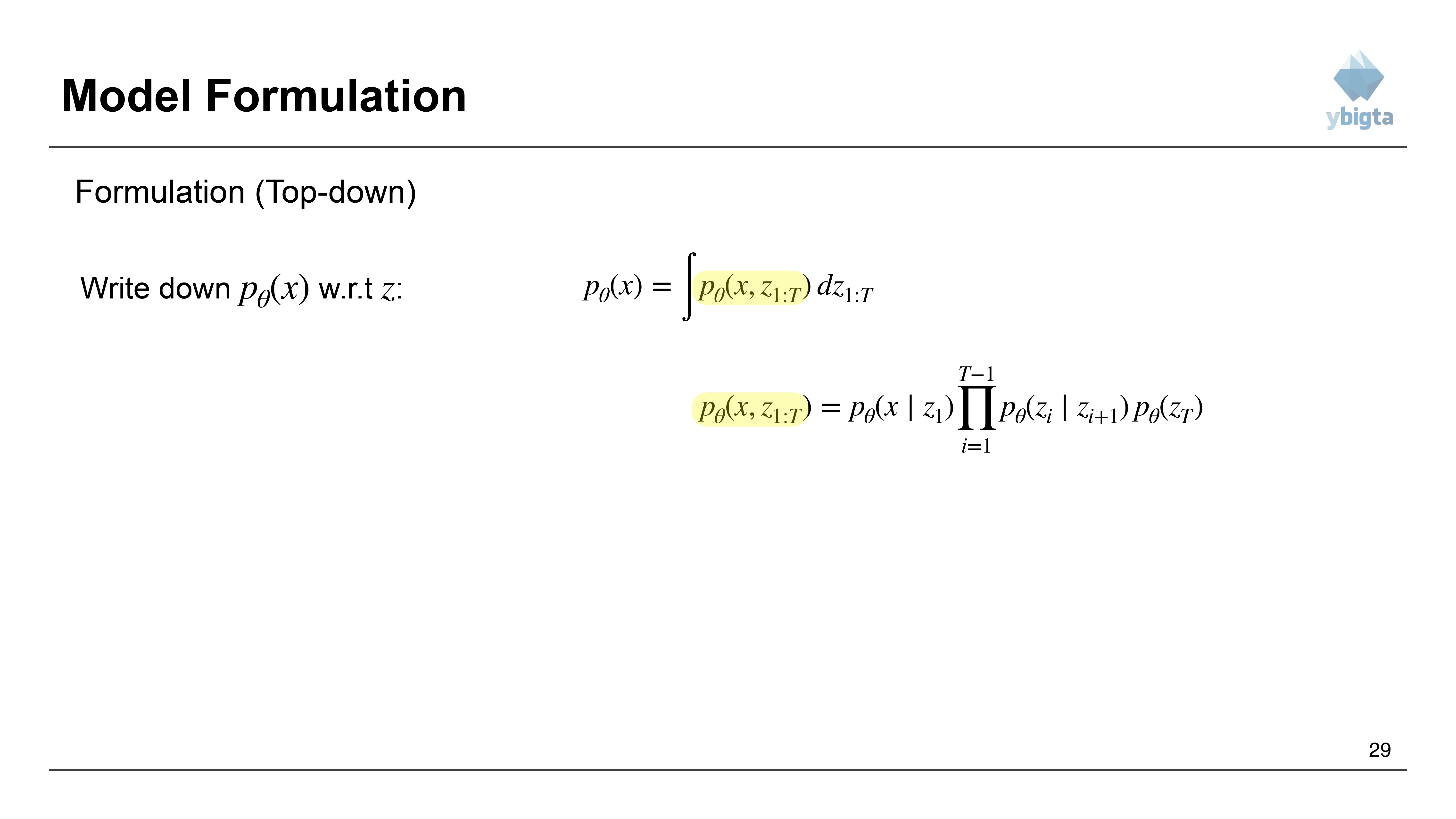
Slide 28: Formulation (Top-down) - Marginalization
- Express $p_\theta(x)$ by marginalizing over all latent steps: $$p_{\theta}(x) = \int p_{\theta}(x, z_{1:T}) dz_{1:T}$$
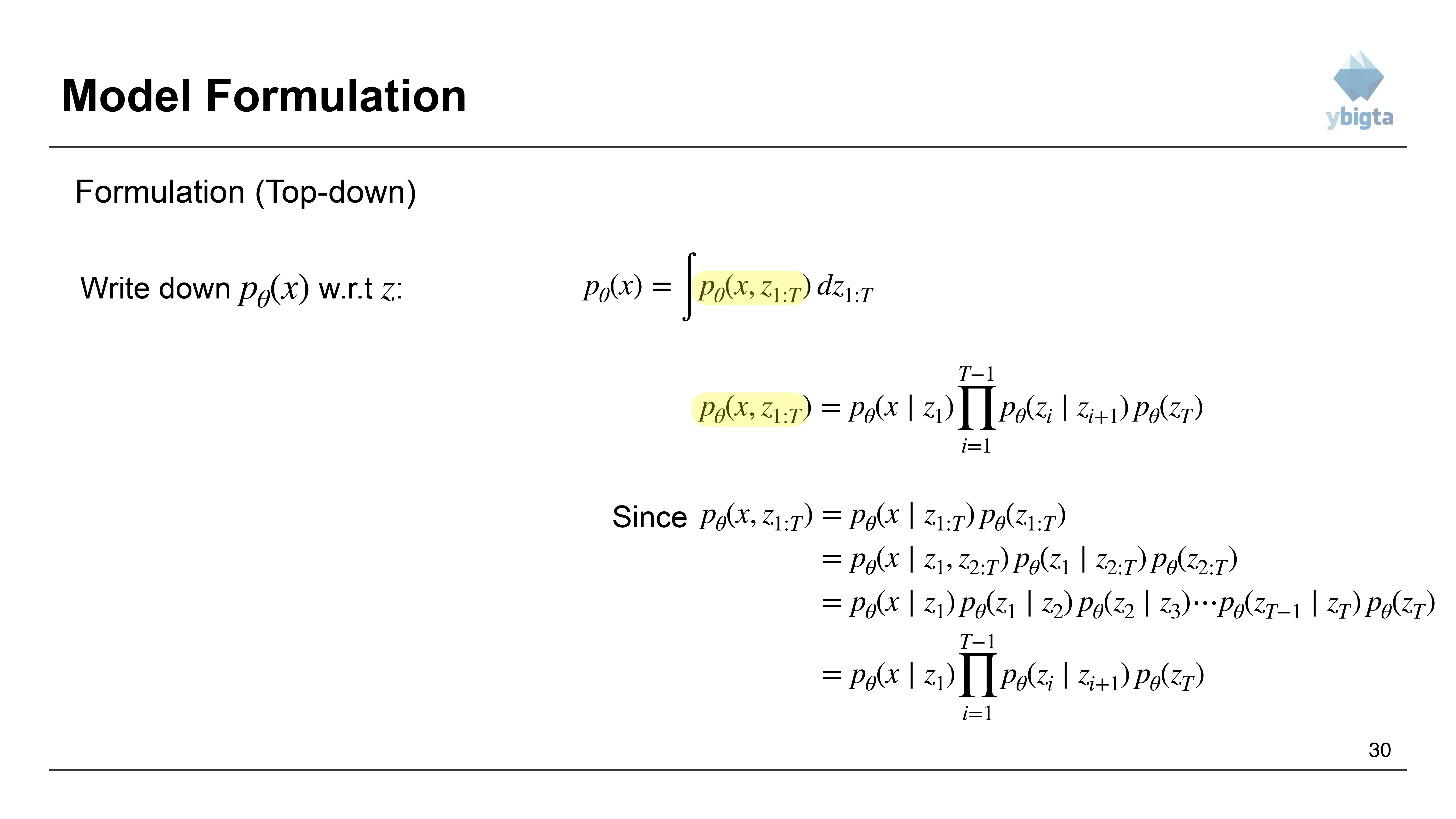
Slide 29: Joint Distribution Expansion
- Expand the joint probability using the chain rule (Markov property): $$p_{\theta}(x, z_{1:T}) = p_{\theta}(x|z_1) \prod_{i=1}^{T-1} p_{\theta}(z_i|z_{i+1}) p_{\theta}(z_T)$$
Slide 30: Detailed Expansion
- Since $p_{\theta}(x, z_{1:T}) = p_{\theta}(x|z_{1:T})p_{\theta}(z_{1:T})$
- By Markov property (dependency only on previous step): $$= p_{\theta}(x|z_1) p_{\theta}(z_1|z_2) p_{\theta}(z_2|z_3) \cdots p_{\theta}(z_{T-1}|z_T) p_{\theta}(z_T)$$ $$= p_{\theta}(x|z_1) \prod_{i=1}^{T-1} p_{\theta}(z_i|z_{i+1}) p_{\theta}(z_T)$$
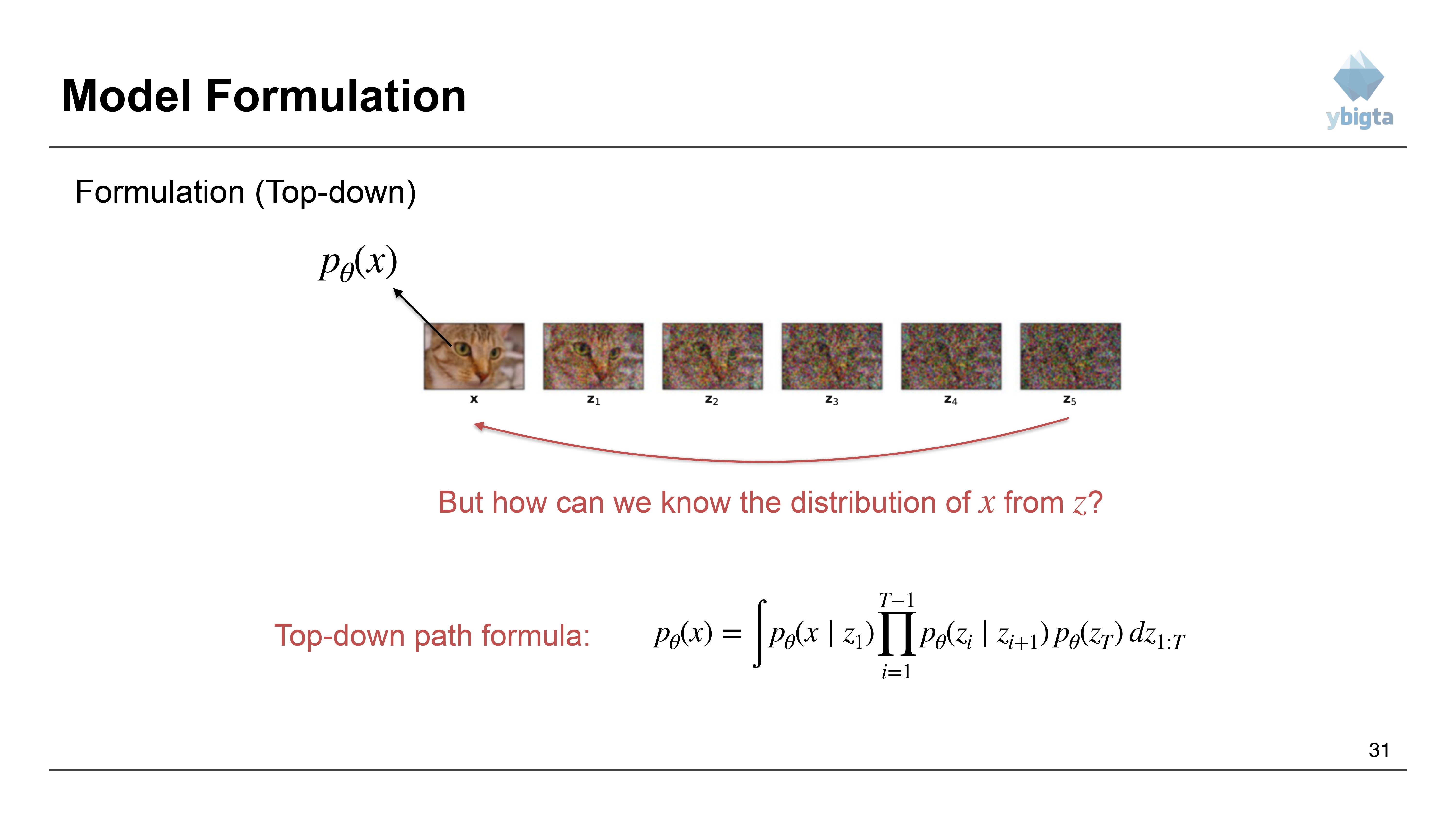
Slide 31: Top-down Path Formula
- Top-down Integral: $$p_{\theta}(x) = \int p_{\theta}(x|z_1) \prod_{i=1}^{T-1} p_{\theta}(z_i|z_{i+1}) p_{\theta}(z_T) dz_{1:T}$$
- This represents the path from Noise ($z_T$) back to Image ($x$).
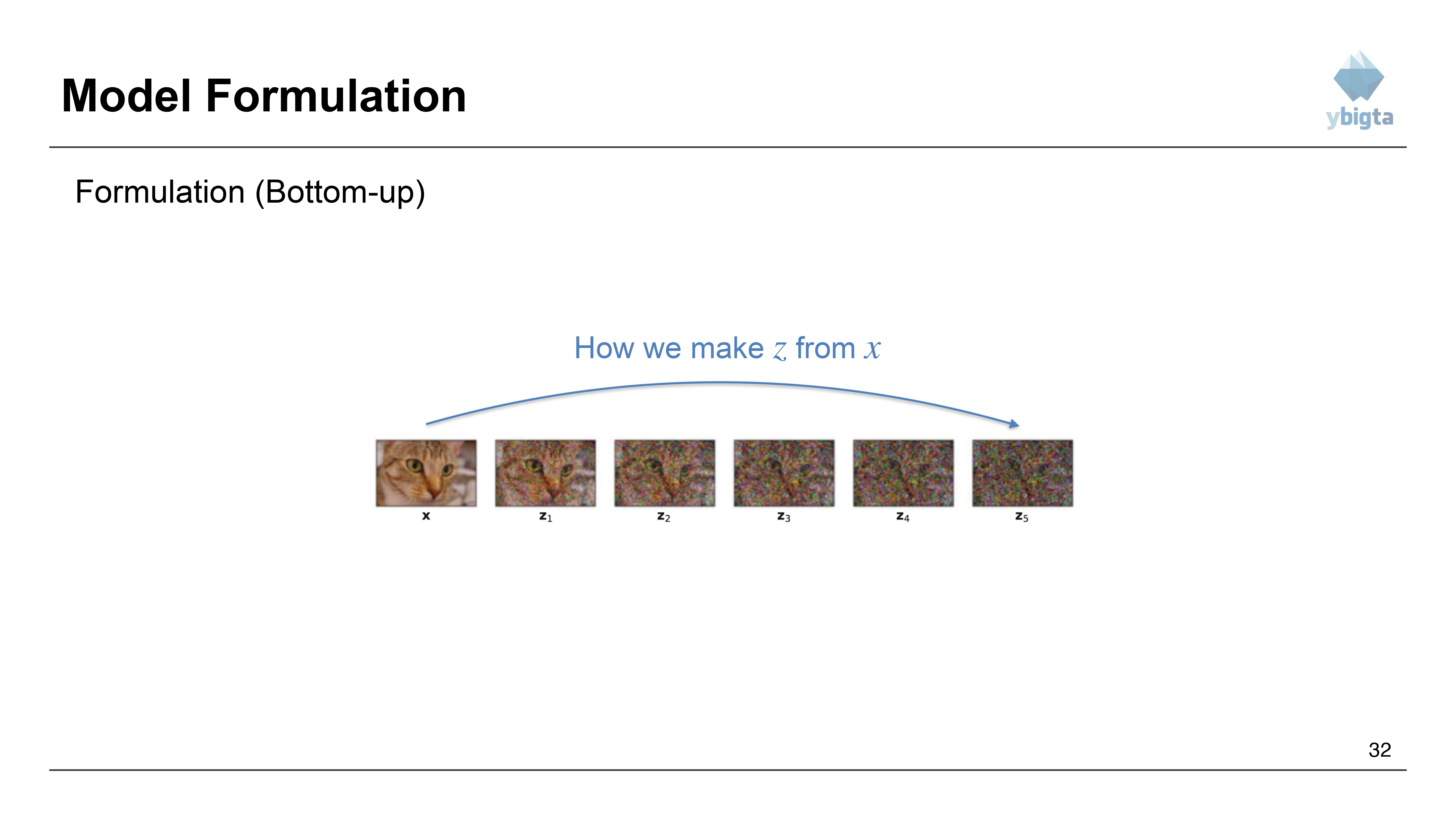
Slide 32: Formulation (Bottom-up)
- Now, how do we make $z$ from $x$ (Forward process)?
- Sequence: $x \to z_1 \to z_2 \dots \to z_5$.
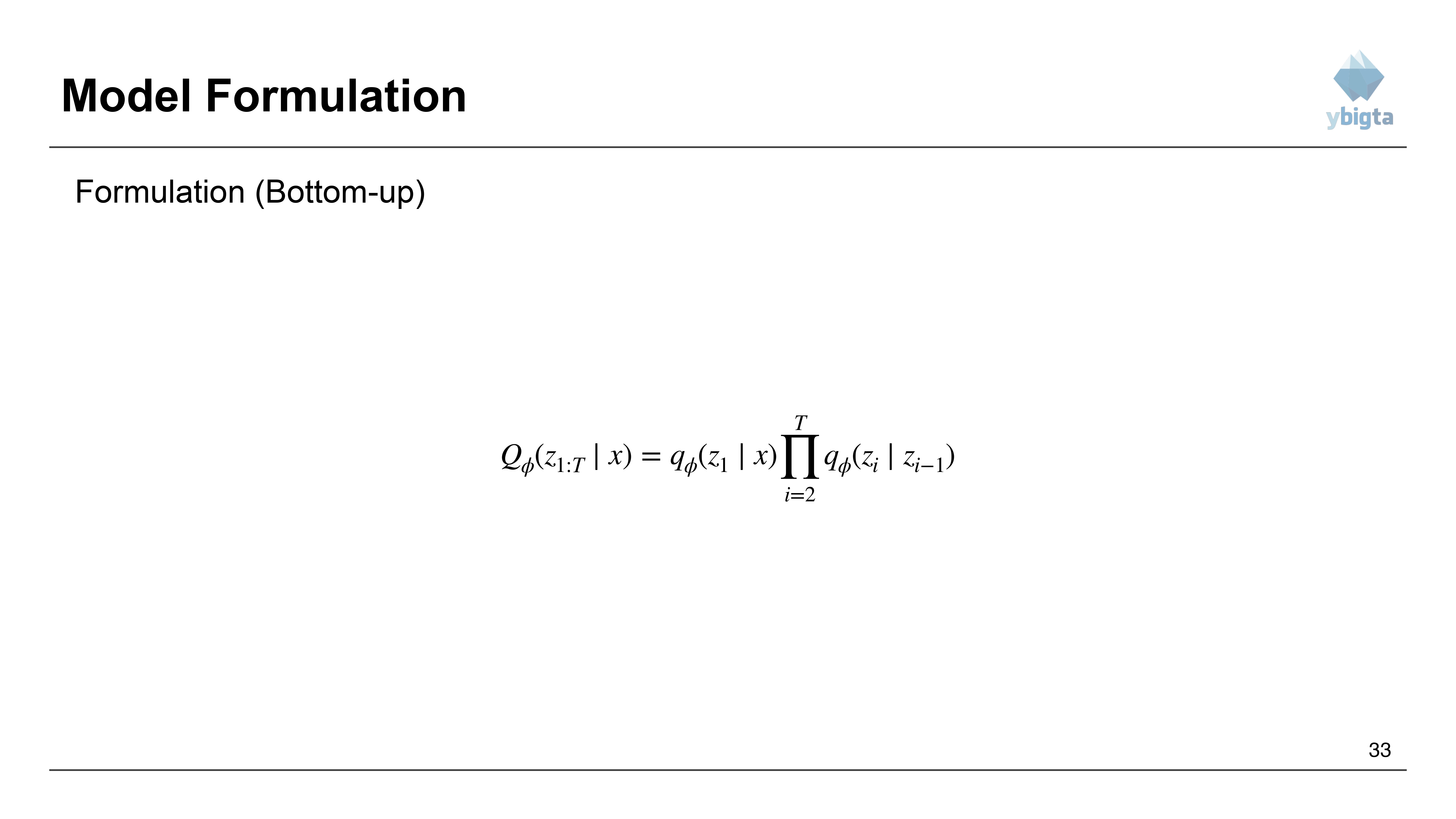
Slide 33: Forward Posterior
- Define the approximate posterior $Q$: $$Q_{\phi}(z_{1:T}|x) = q_{\phi}(z_1|x) \prod_{i=2}^{T} q_{\phi}(z_i|z_{i-1})$$
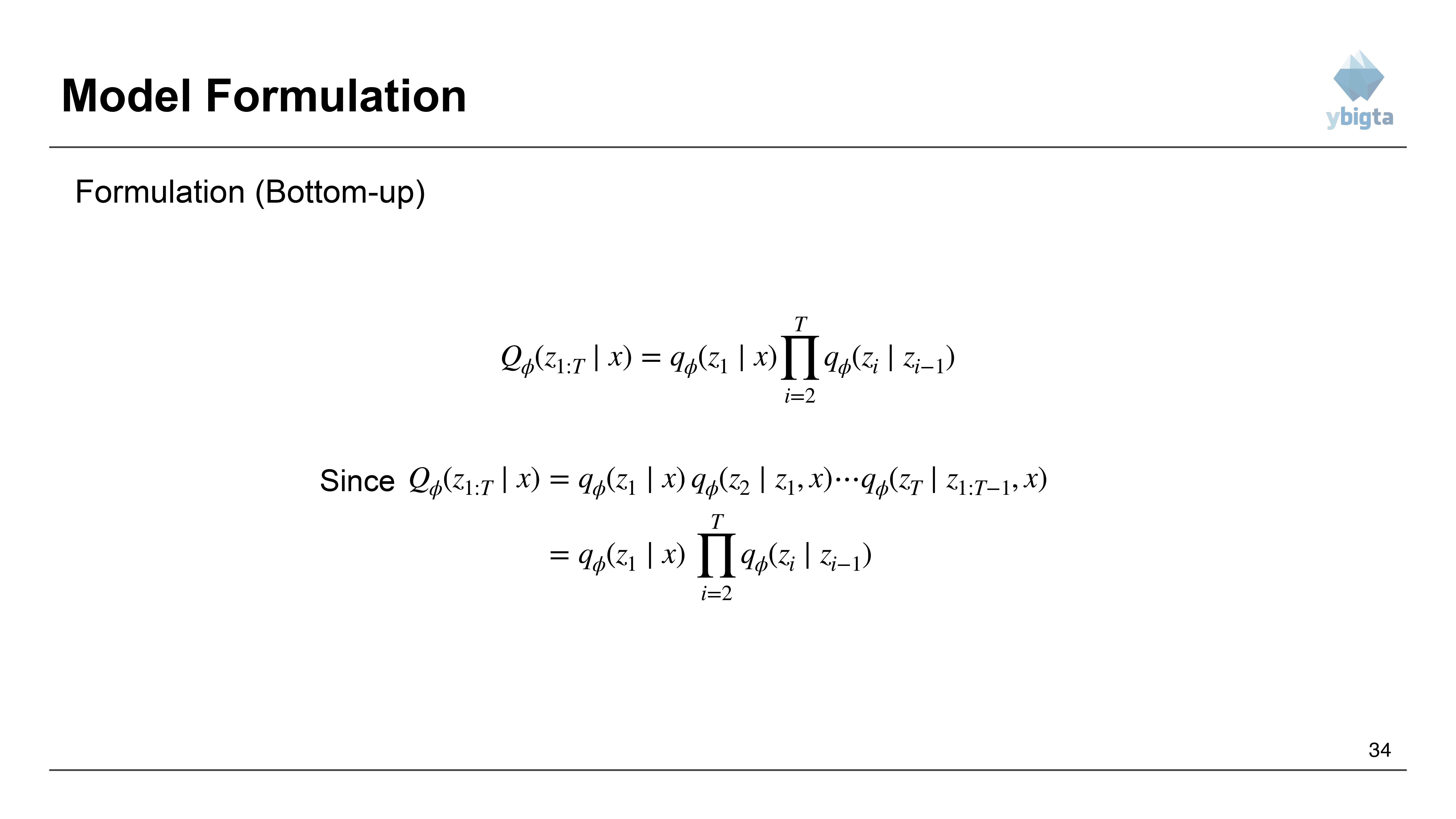
Slide 34: Forward Chain Expansion
- Breaking down the joint posterior: $$Q_{\phi}(z_{1:T}|x) = q_{\phi}(z_1|x) q_{\phi}(z_2|z_1, x) \cdots q_{\phi}(z_T|z_{1:T-1}, x)$$
- Utilizing Markov property: $$= q_{\phi}(z_1|x) \prod_{i=2}^{T} q_{\phi}(z_i|z_{i-1})$$
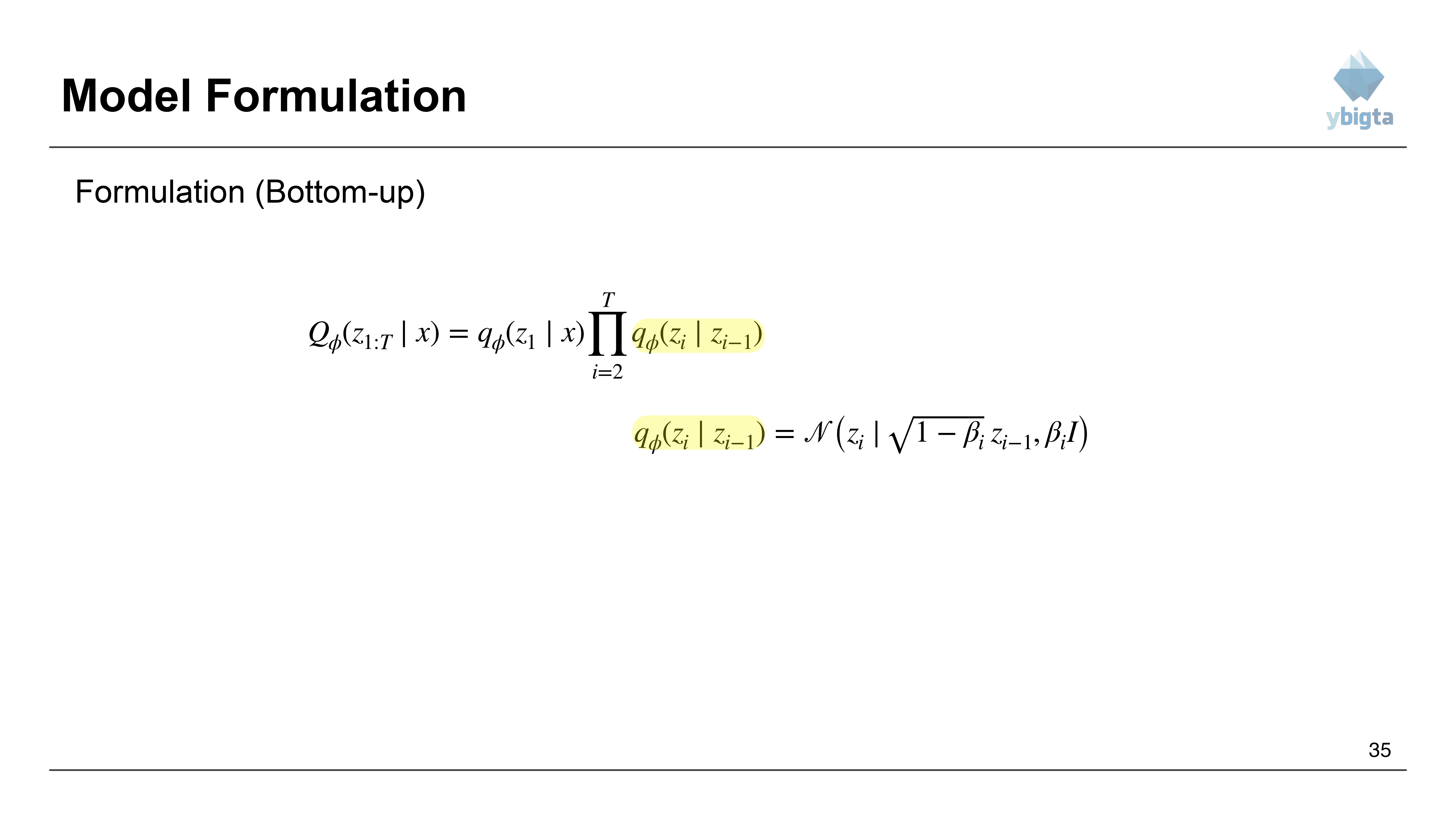
Slide 35: Defining the Transition Kernel
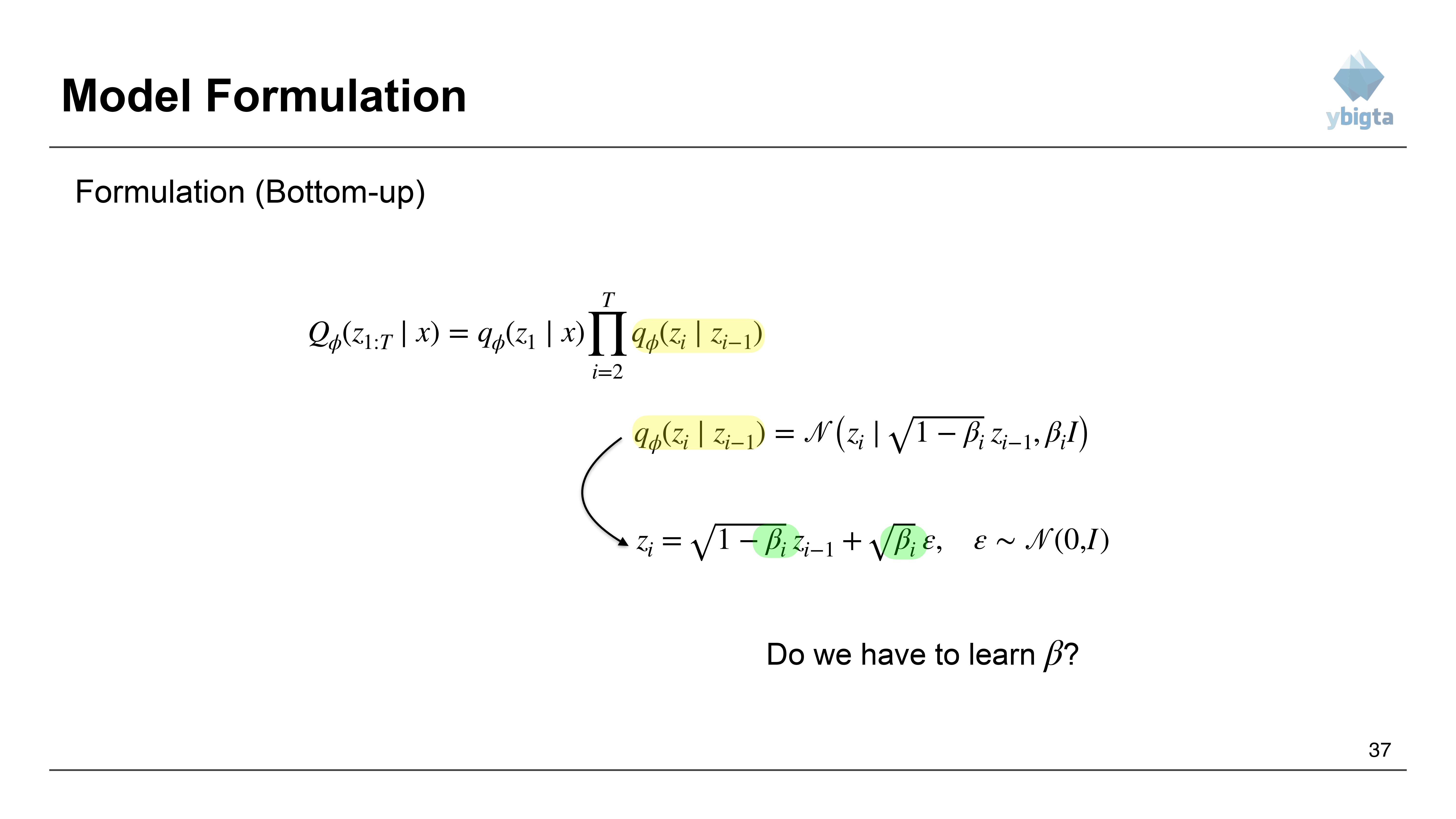
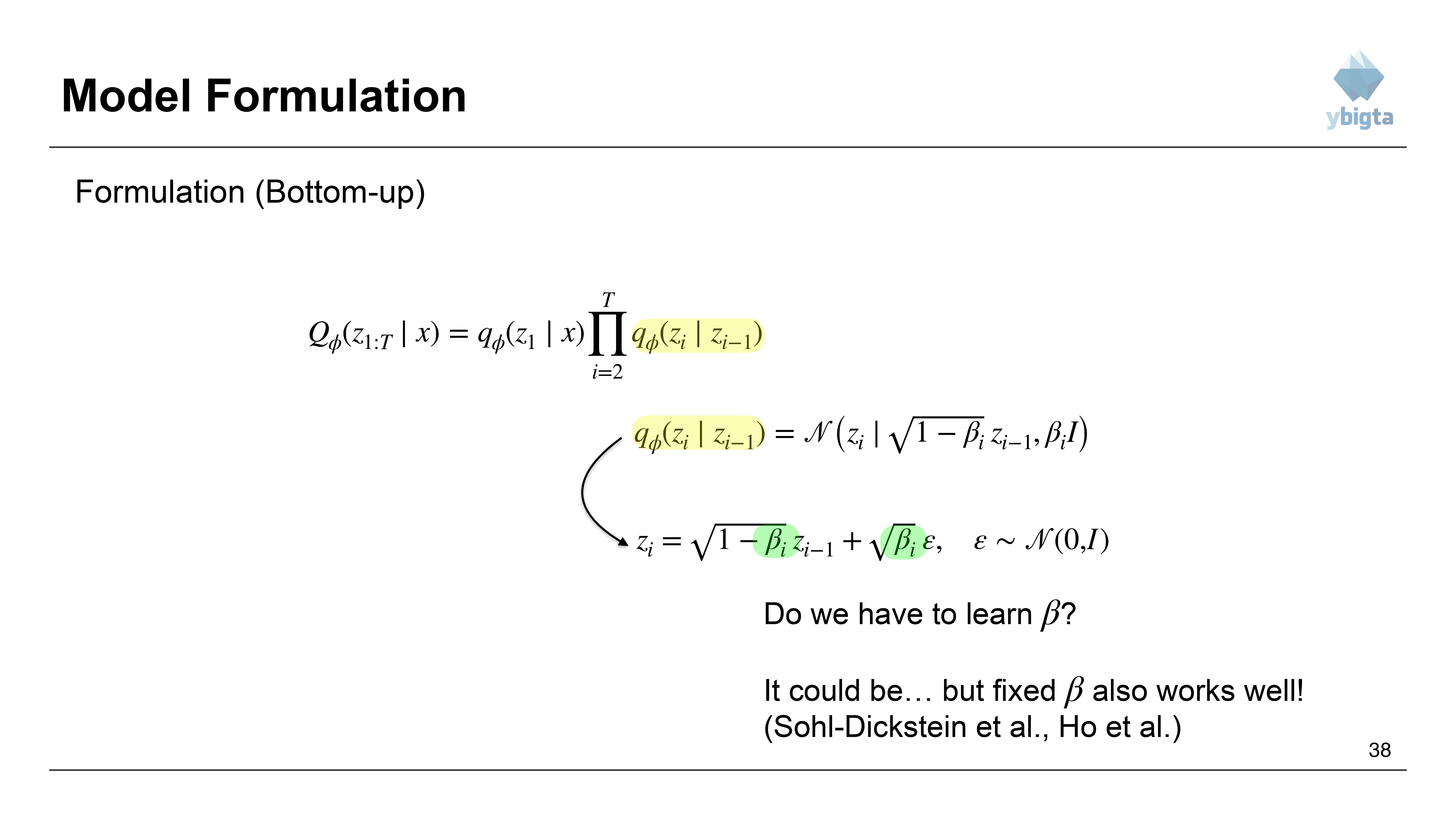
- The forward step is defined as adding Gaussian noise: $$q_{\phi}(z_i|z_{i-1}) = \mathcal{N}(z_i | \sqrt{1-\beta_i}z_{i-1}, \beta_i I)$$
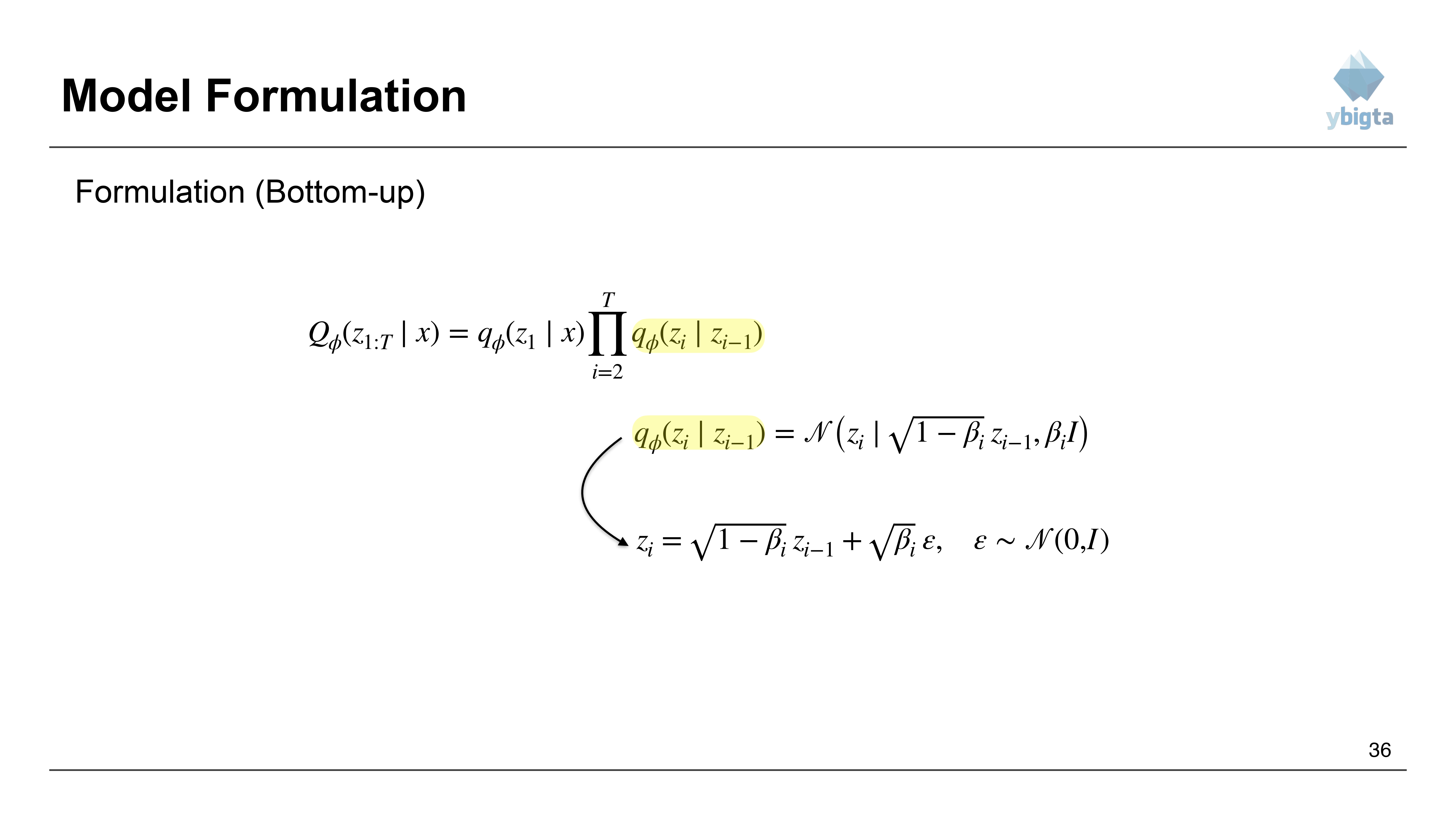
Slide 36: Reparameterization
- Using the reparameterization trick: $$z_i = \sqrt{1-\beta_i}z_{i-1} + \sqrt{\beta_i}\epsilon, \quad \epsilon \sim \mathcal{N}(0, I)$$
Slide 37: Learning $\beta$?
- Question: Do we have to learn the schedule of $\beta_i$?
Slide 38: Fixed Variance
- Answer: It could be learned, but fixed $\beta$ also works well!
- References: Sohl-Dickstein et al., Ho et al.
Slide 39: Overall Formulation Summary
- Bottom-up (Encoder/Forward): $$Q_{\phi}(z_{1:T}|x) = q_{\phi}(z_1|x) \prod_{i=2}^{T} q_{\phi}(z_i|z_{i-1})$$ $$z_i = \sqrt{1-\beta_i}z_{i-1} + \sqrt{\beta_i}\epsilon$$
- Top-down (Decoder/Reverse): $$p_{\theta}(x) = \int p_{\theta}(x|z_1) \prod_{i=1}^{T-1} p_{\theta}(z_i|z_{i+1}) p_{\theta}(z_T) dz_{1:T}$$
Slide 40: Where are the Learnable Parameters?
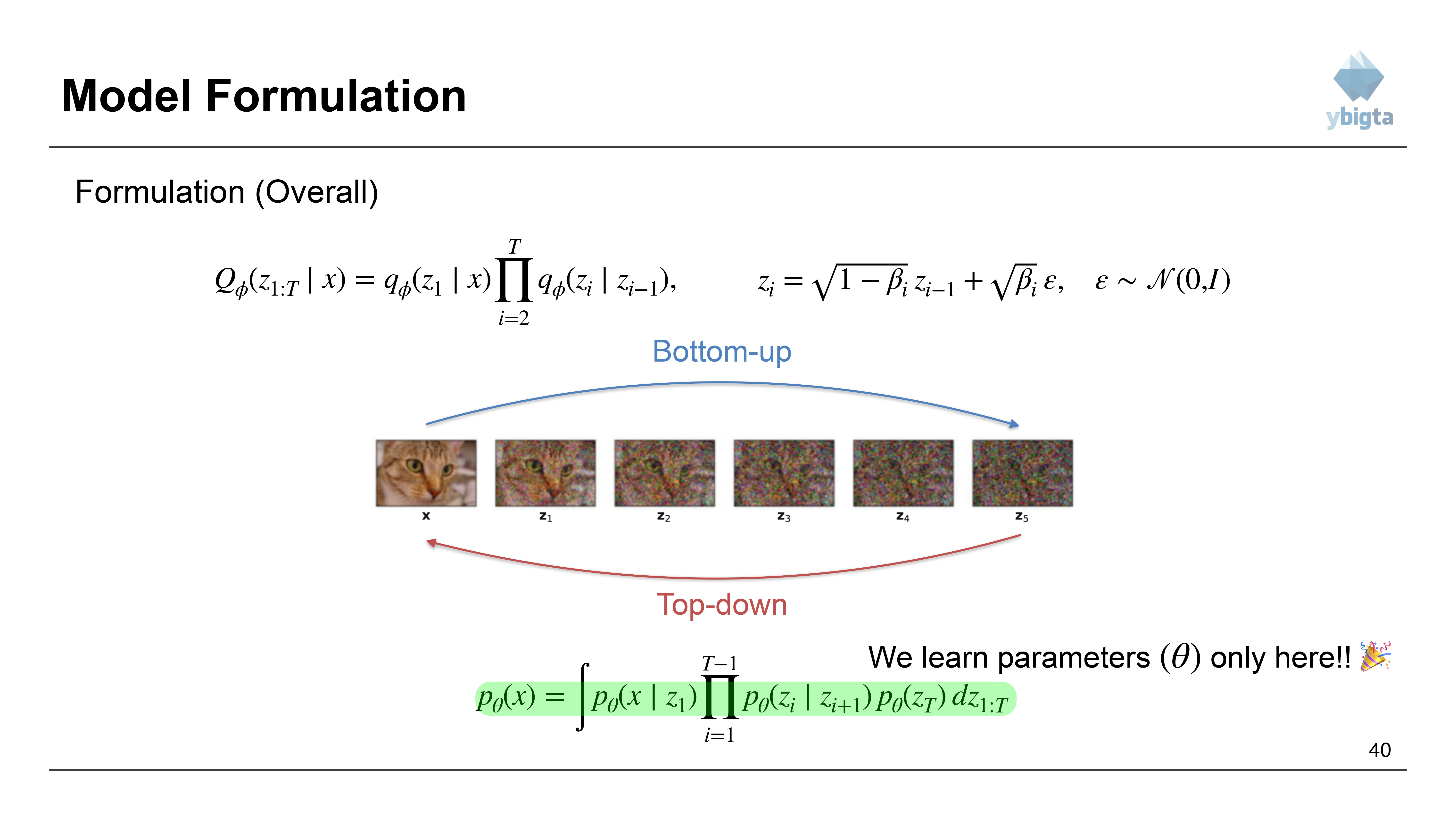
- Bottom-up: Fixed (Gaussian noise).
- Top-down: Parameters $\theta$ exist here! We need to learn the reverse process.
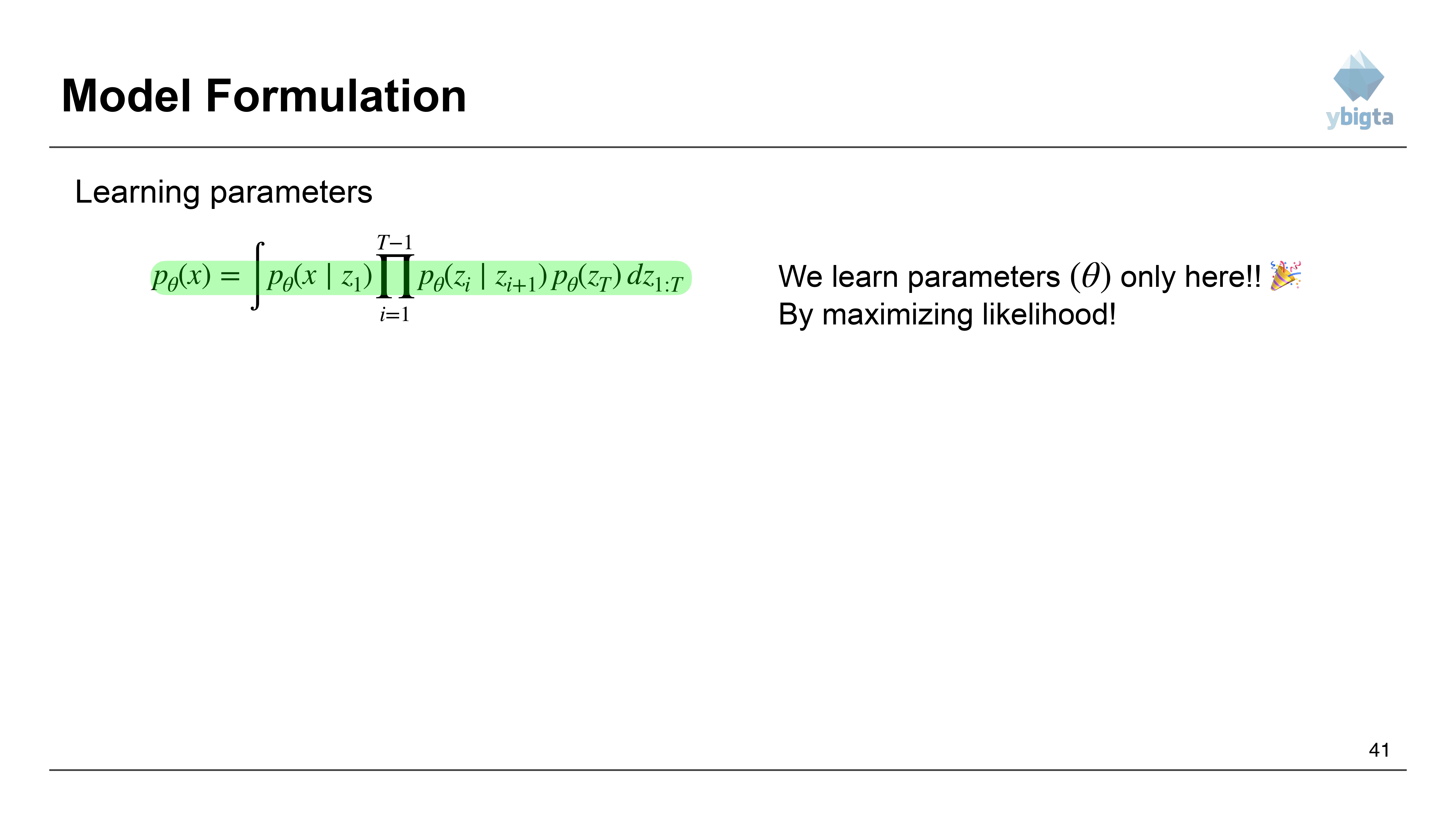
Slide 41: Learning Parameters
- We learn parameters $\theta$ by maximizing likelihood.
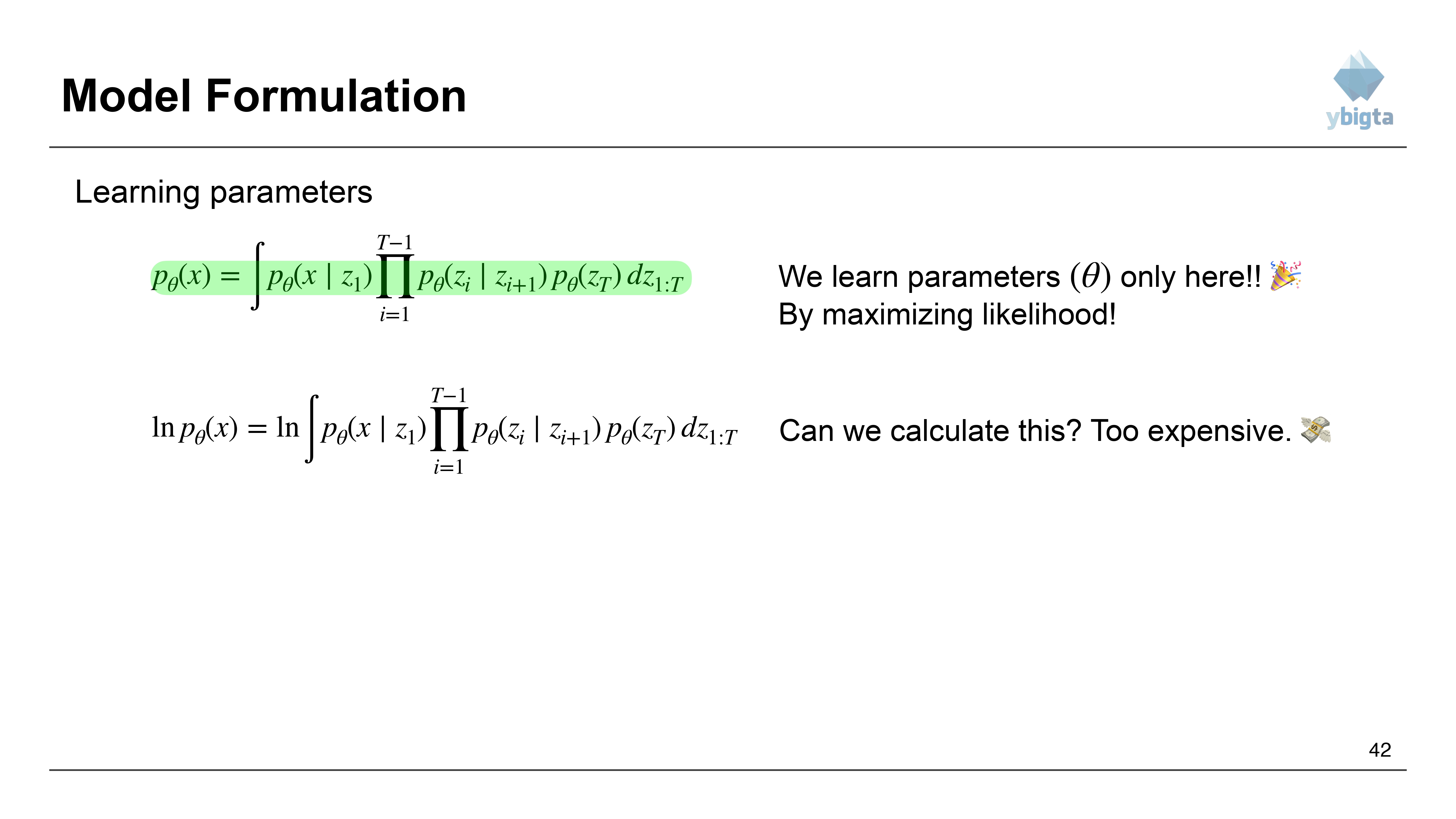
Slide 42: Intractability
- Objective: Maximize $\ln p_{\theta}(x)$.
- $$\ln p_{\theta}(x) = \ln \int p_{\theta}(x|z_1) \prod_{i=1}^{T-1} p_{\theta}(z_i|z_{i+1}) p_{\theta}(z_T) dz_{1:T}$$
- Problem: Can we calculate this integral? No, it’s too expensive (intractable).
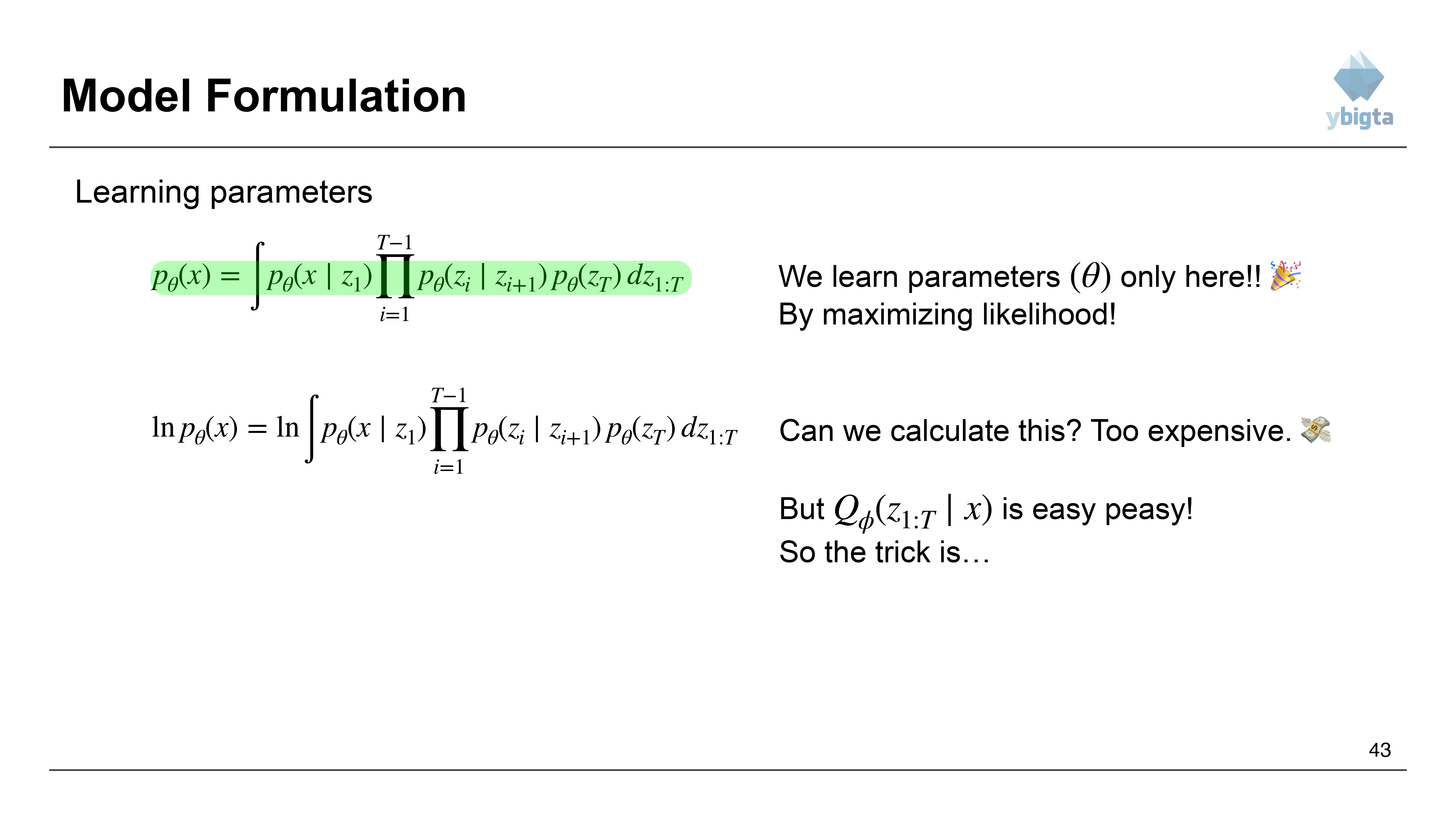
Slide 43: The Trick
- However, the forward process $Q_{\phi}(z_{1:T}|x)$ is “easy peasy” (just adding noise).
- We can use this to approximate the objective.
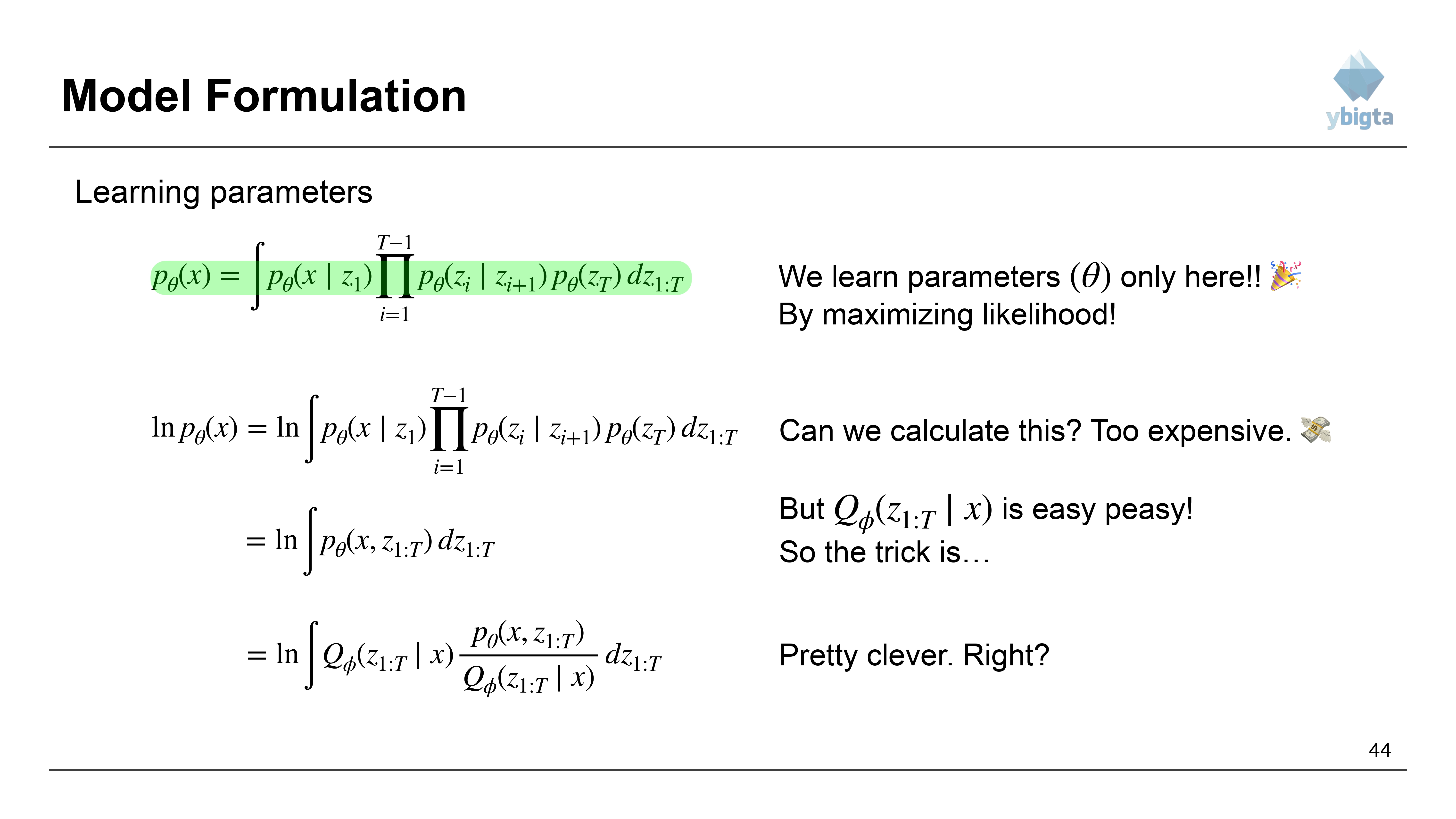
Slide 44: Importance Sampling Setup
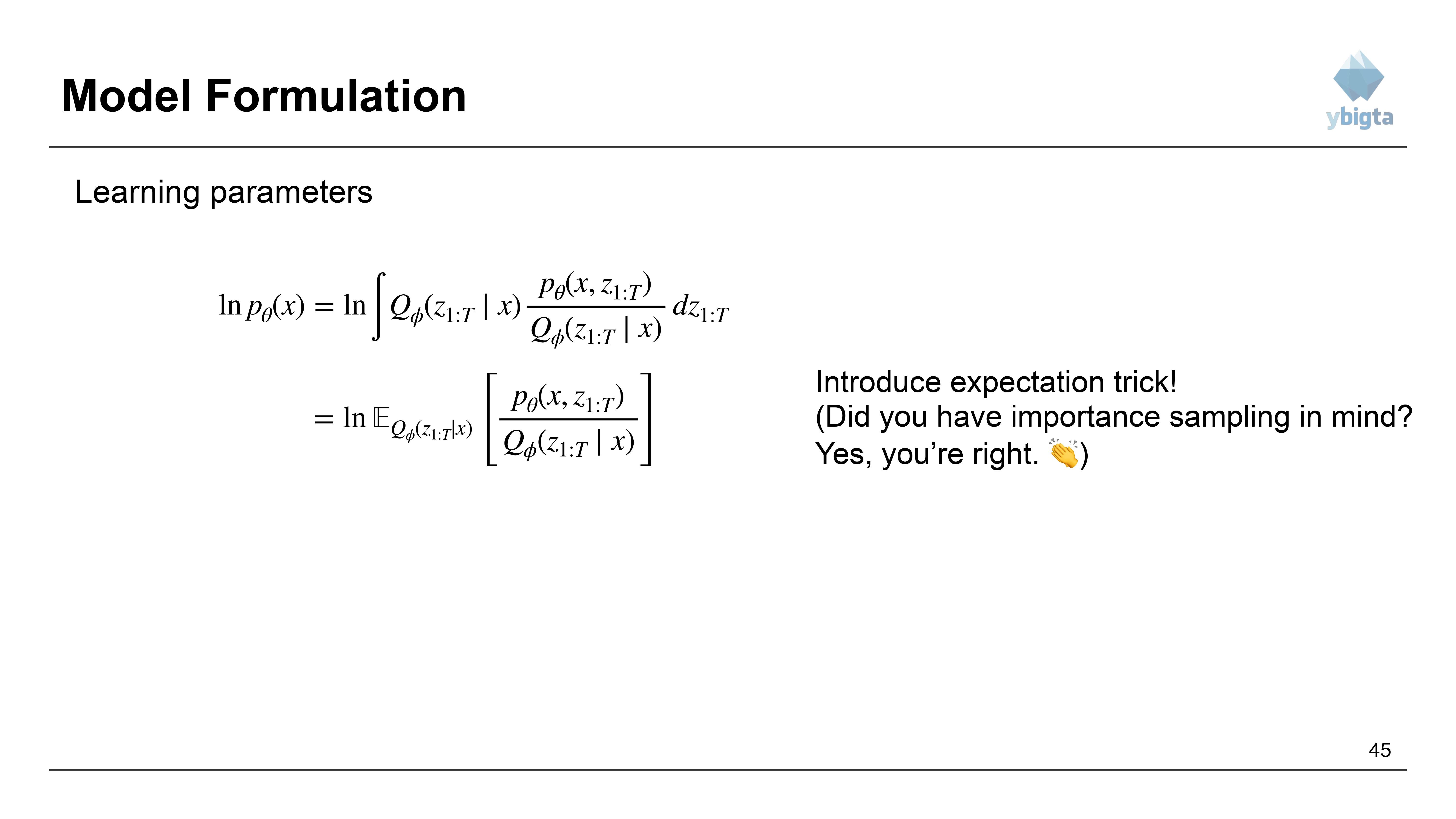
- Multiply and divide by $Q$: $$= \ln \int Q_{\phi}(z_{1:T}|x) \frac{p_{\theta}(x, z_{1:T})}{Q_{\phi}(z_{1:T}|x)} dz_{1:T}$$
Slide 45: Expectation Form
- Convert integral to expectation: $$= \ln E_{Q_{\phi}(z_{1:T}|x)} \left[ \frac{p_{\theta}(x, z_{1:T})}{Q_{\phi}(z_{1:T}|x)} \right]$$
- This is related to Importance Sampling.
Slide 46: Jensen’s Inequality
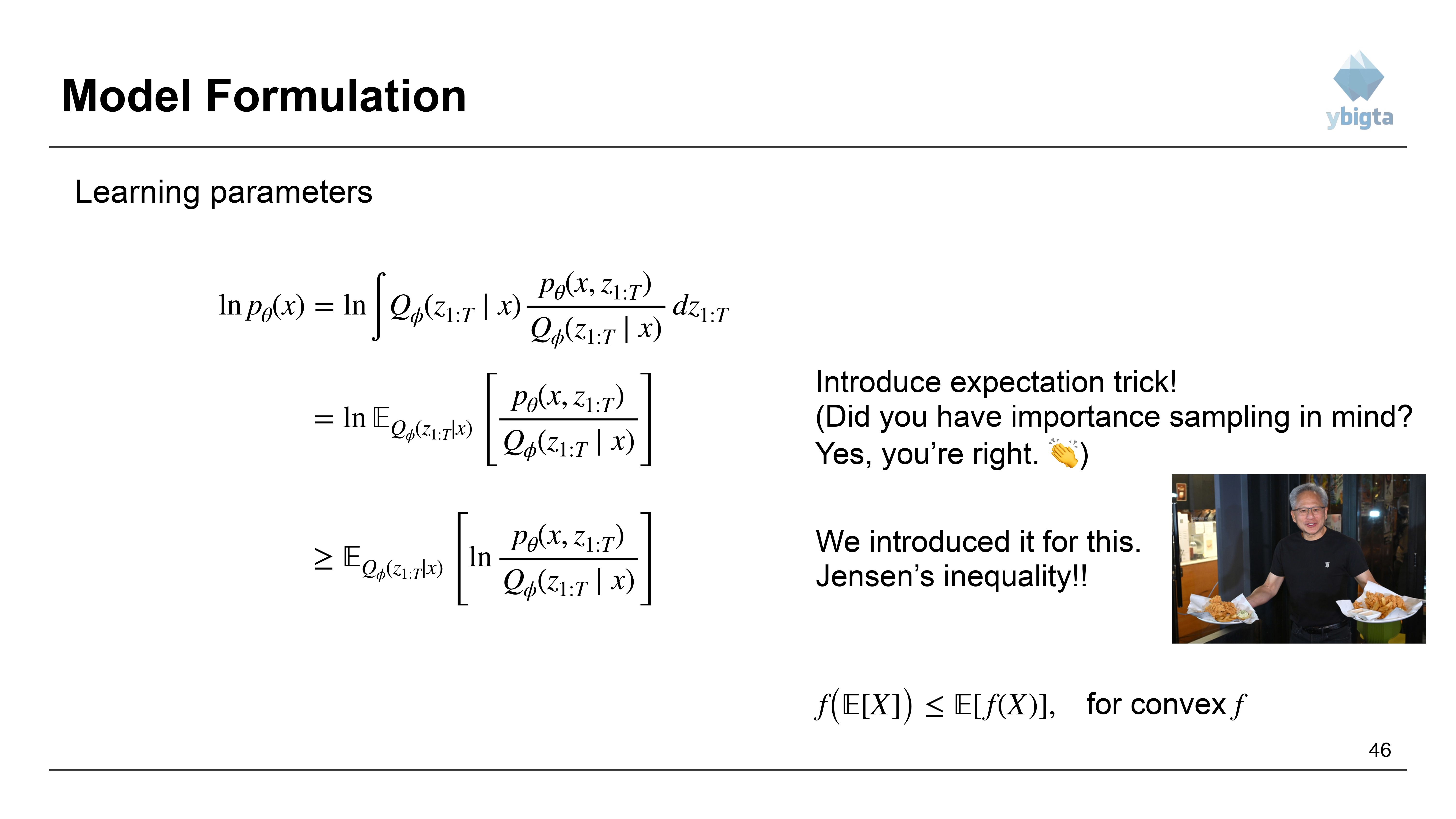
- We use Jensen’s Inequality: $f(\mathbb{E}[X]) \le \mathbb{E}[f(X)]$ for convex $f$ (or $\ge$ for concave like $\ln$).
- $$\ge E_{Q_{\phi}(z_{1:T}|x)} \left[ \ln \frac{p_{\theta}(x, z_{1:T})}{Q_{\phi}(z_{1:T}|x)} \right]$$
Slide 47: The Lower Bound
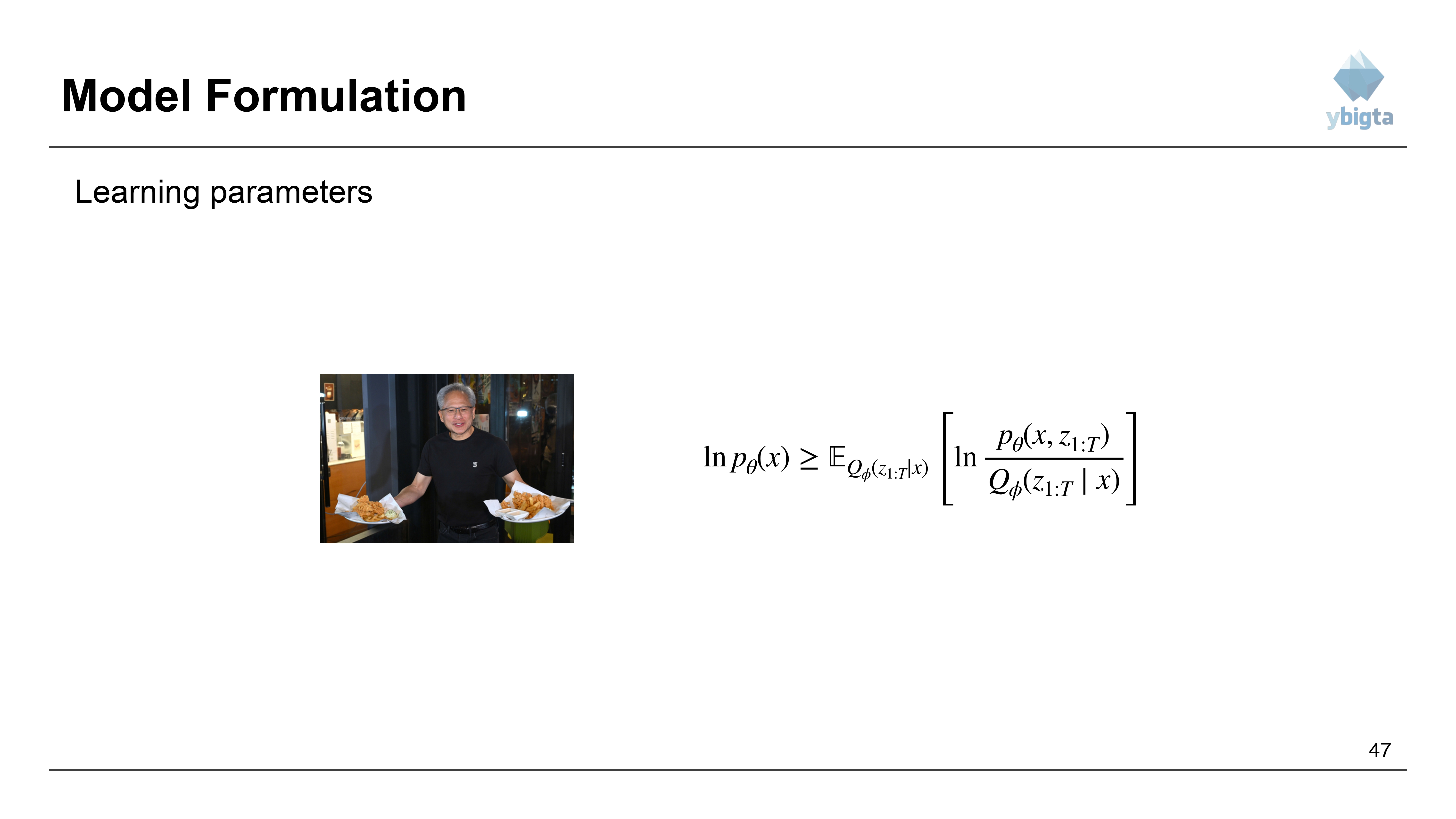
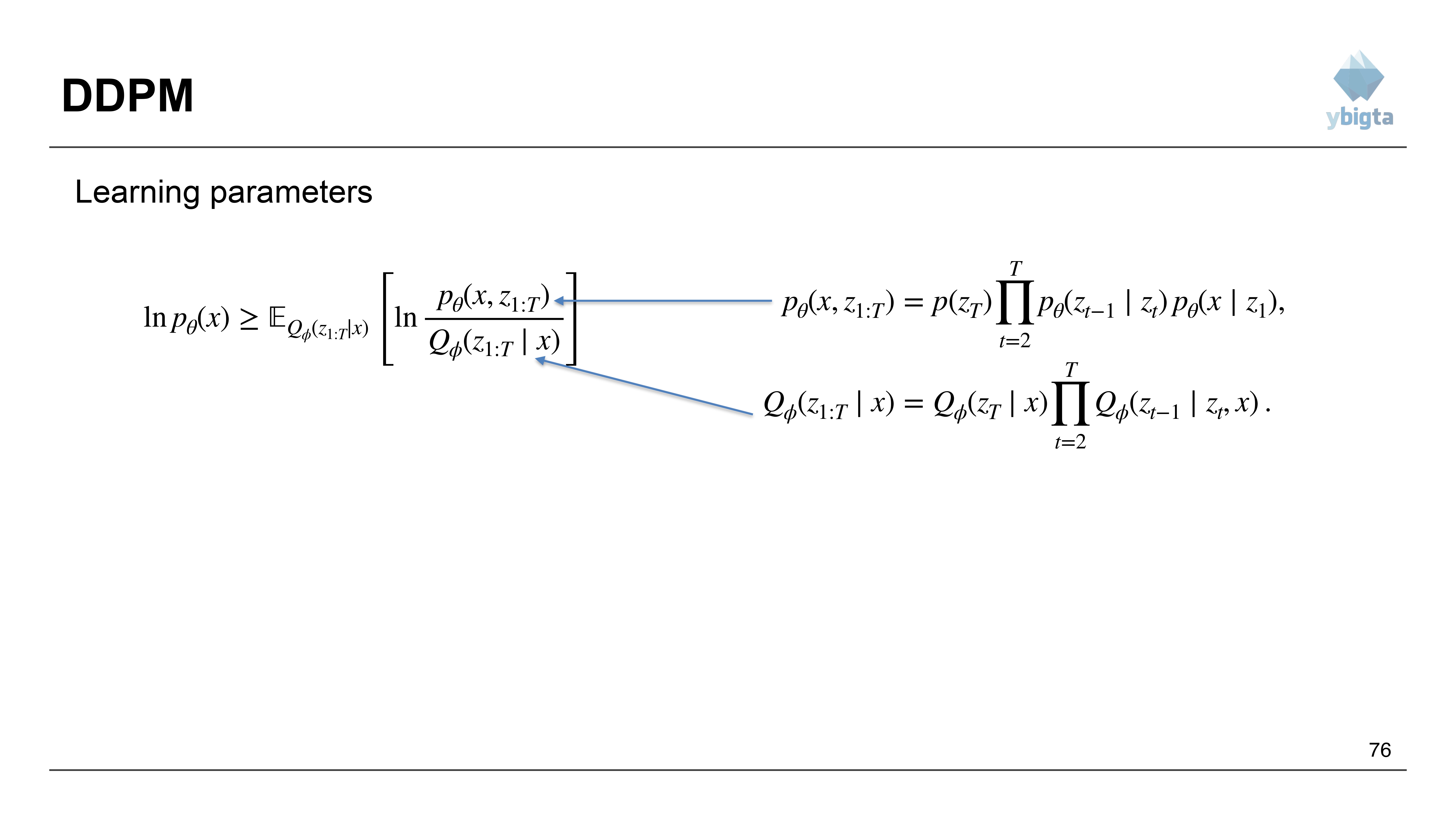
- We now have a lower bound on the log-likelihood: $$\ln p_{\theta}(x) \ge E_{Q_{\phi}(z_{1:T}|x)} \left[ \ln \frac{p_{\theta}(x, z_{1:T})}{Q_{\phi}(z_{1:T}|x)} \right]$$
Slide 48: Expanding the Terms
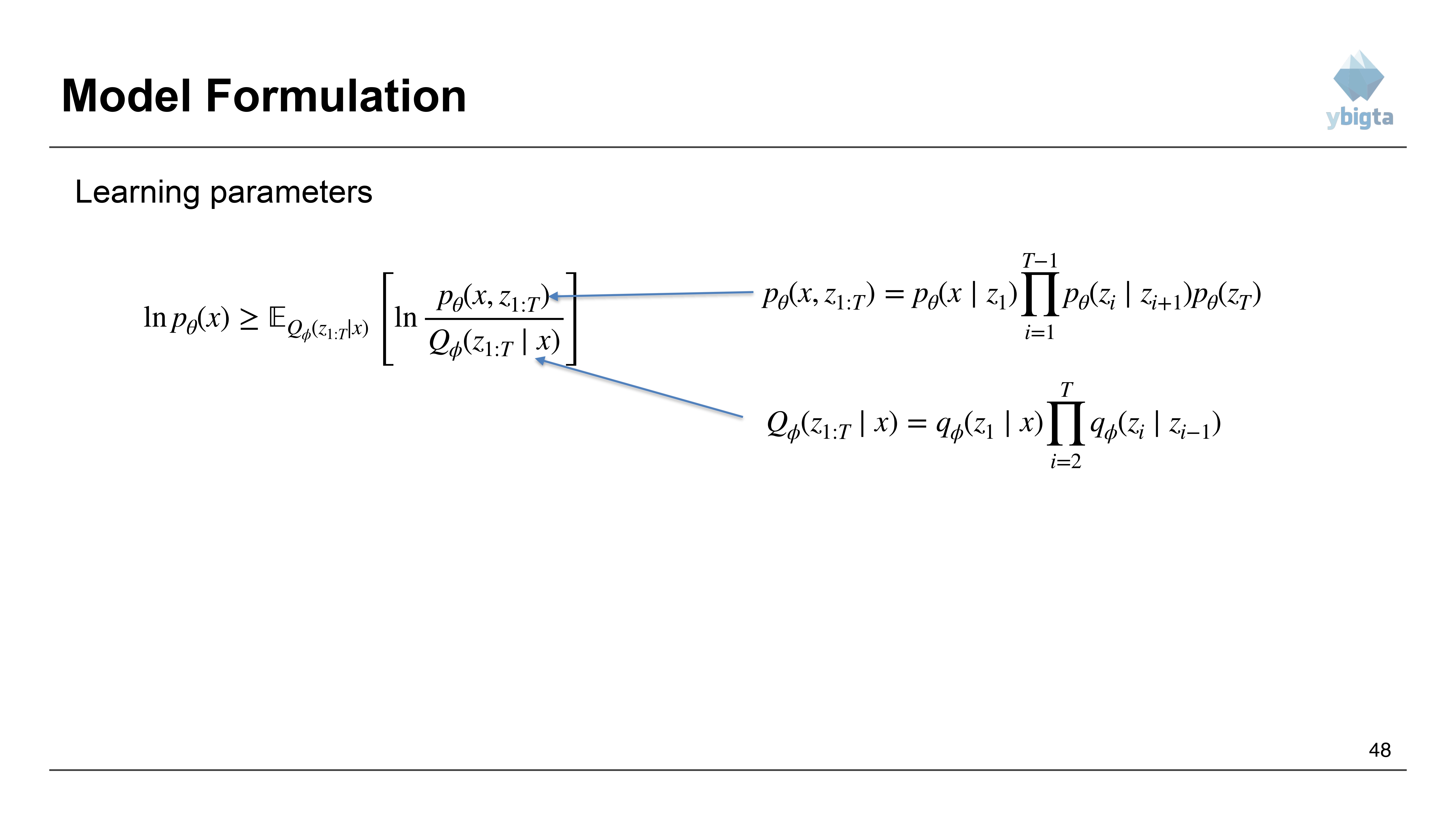
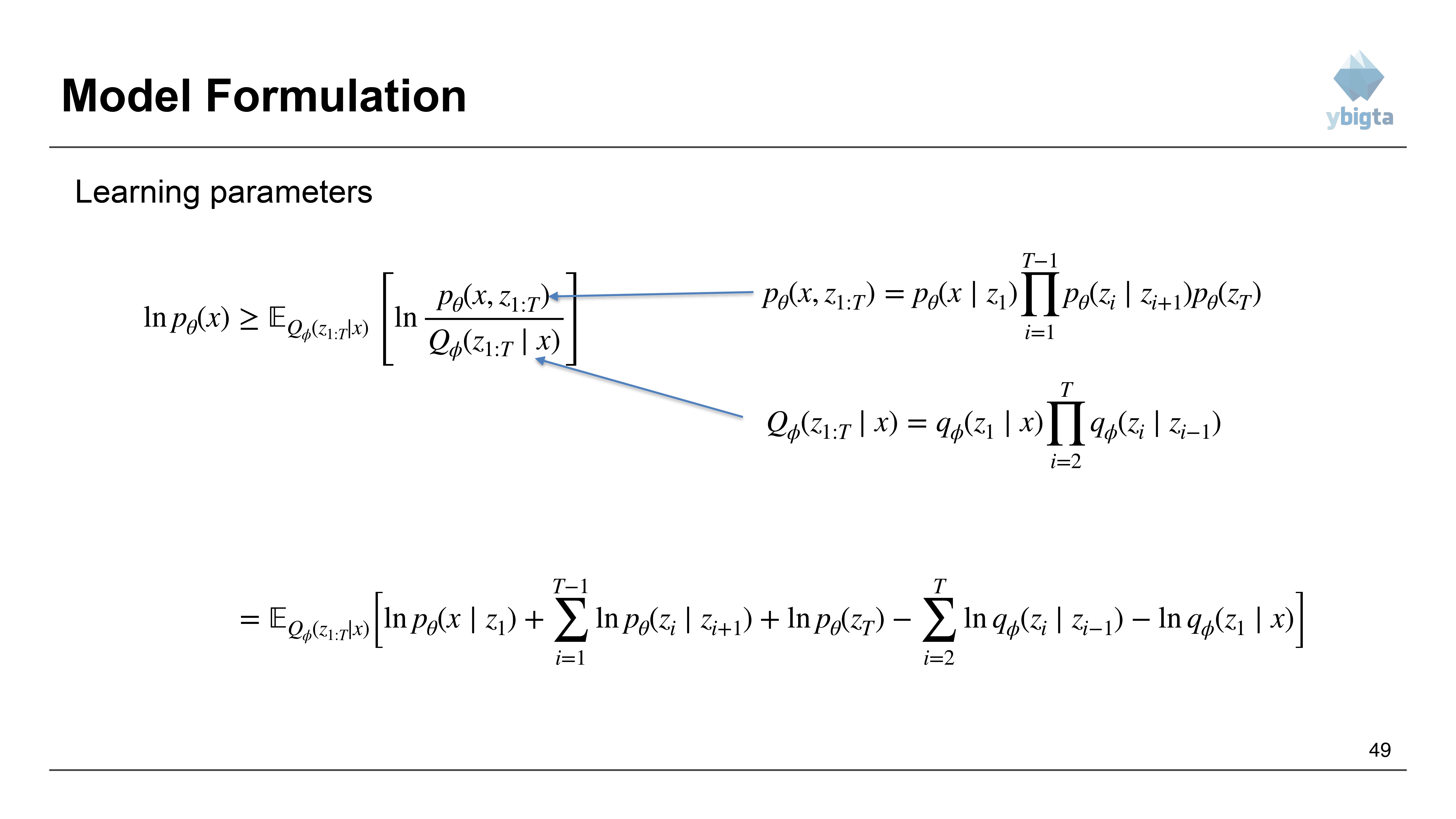
- Substitute the definitions of $p_{\theta}$ (reverse) and $Q_{\phi}$ (forward): $$p_{\theta}(x, z_{1:T}) = p_{\theta}(x|z_1) \prod_{i=1}^{T-1} p_{\theta}(z_i|z_{i+1}) p_{\theta}(z_T)$$ $$Q_{\phi}(z_{1:T}|x) = q_{\phi}(z_1|x) \prod_{i=2}^{T} q_{\phi}(z_i|z_{i-1})$$
Slide 49: Log Expansion (1)
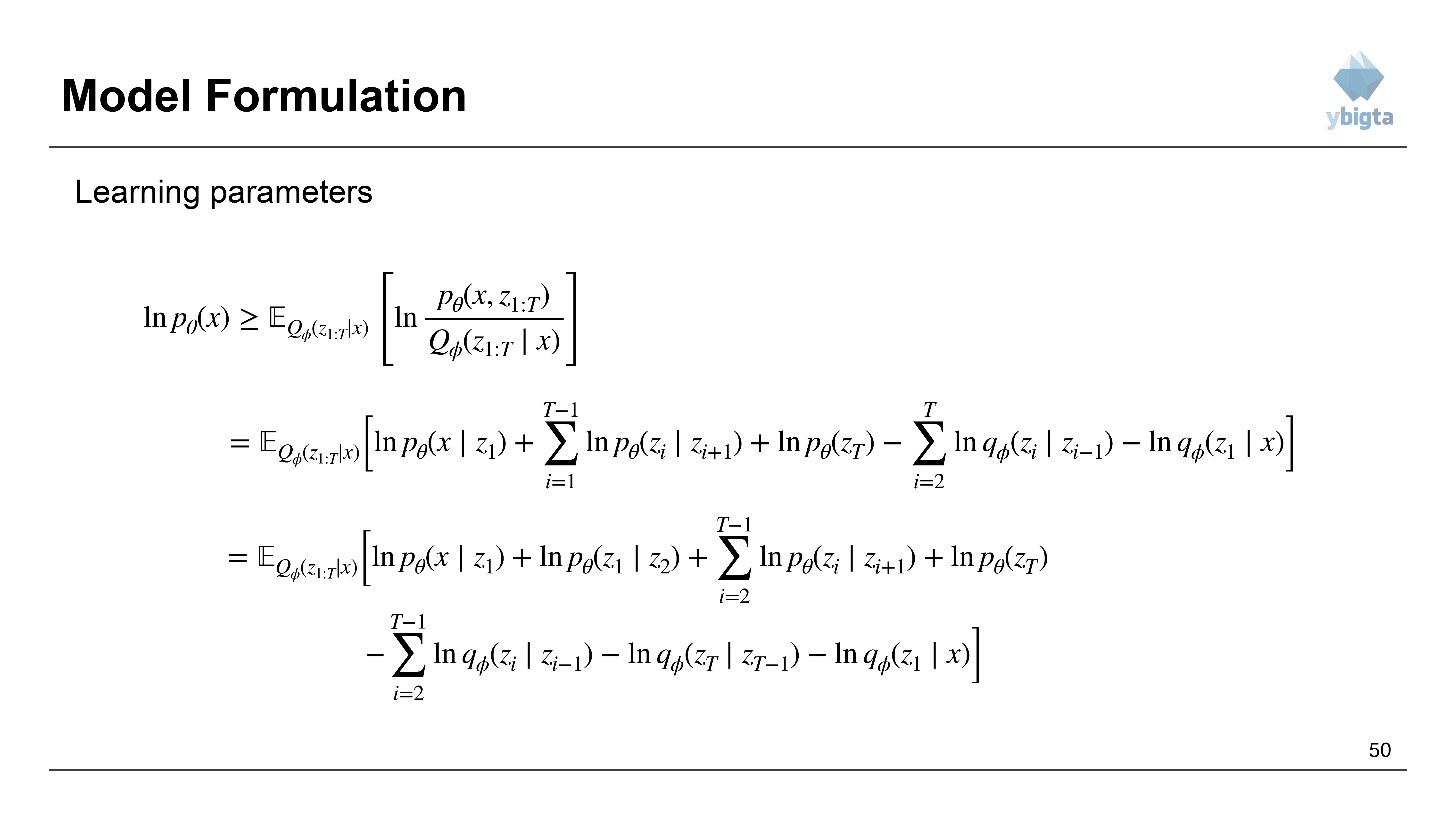
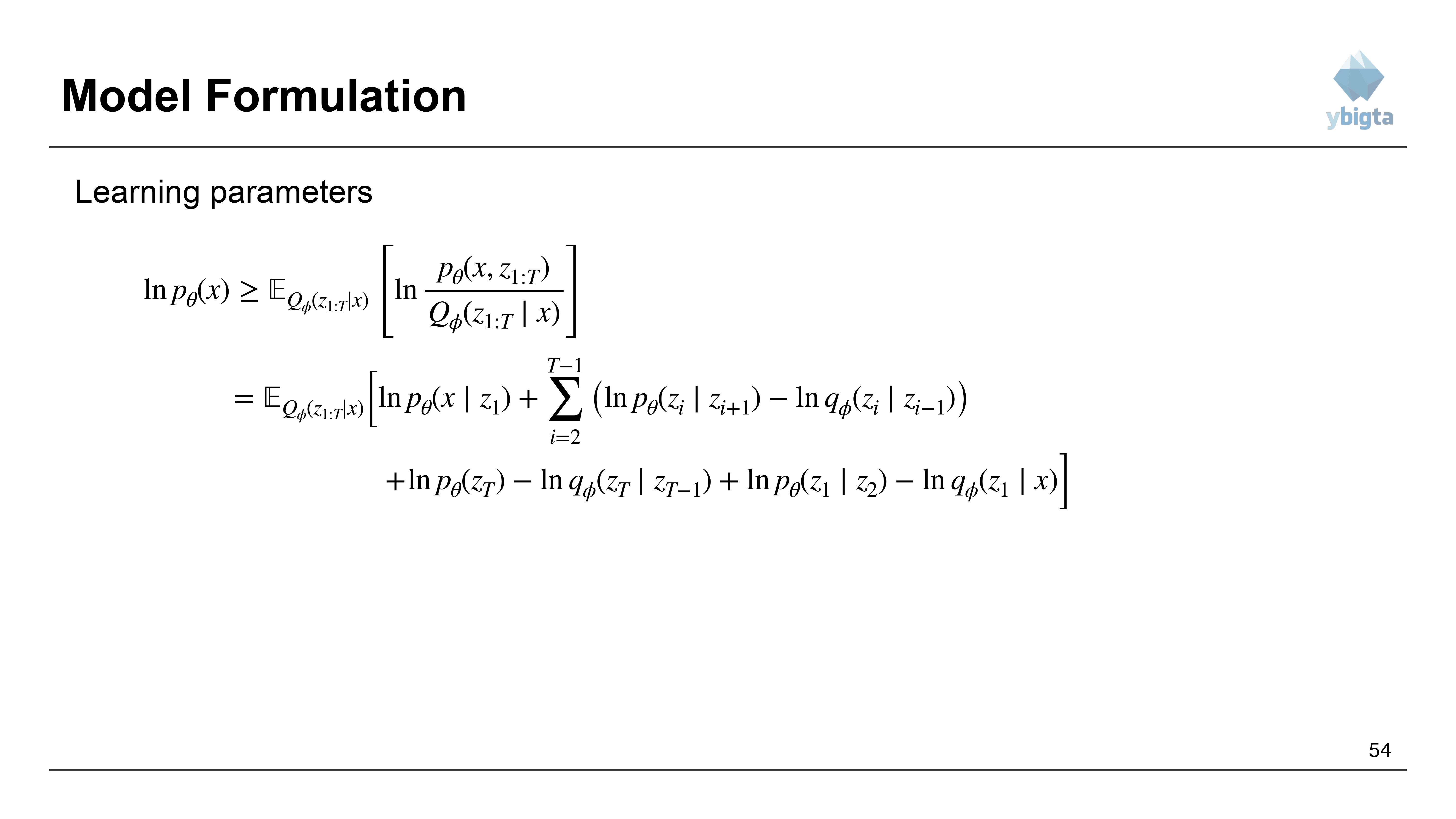
- Expanding the log term inside the expectation: $$E_{Q_{\phi}} [\ln p_{\theta}(x|z_1) + \sum \ln p_{\theta} - \sum \ln q_{\phi} - \ln q_{\phi}(z_1|x)]$$
Slide 50: Log Expansion (2)
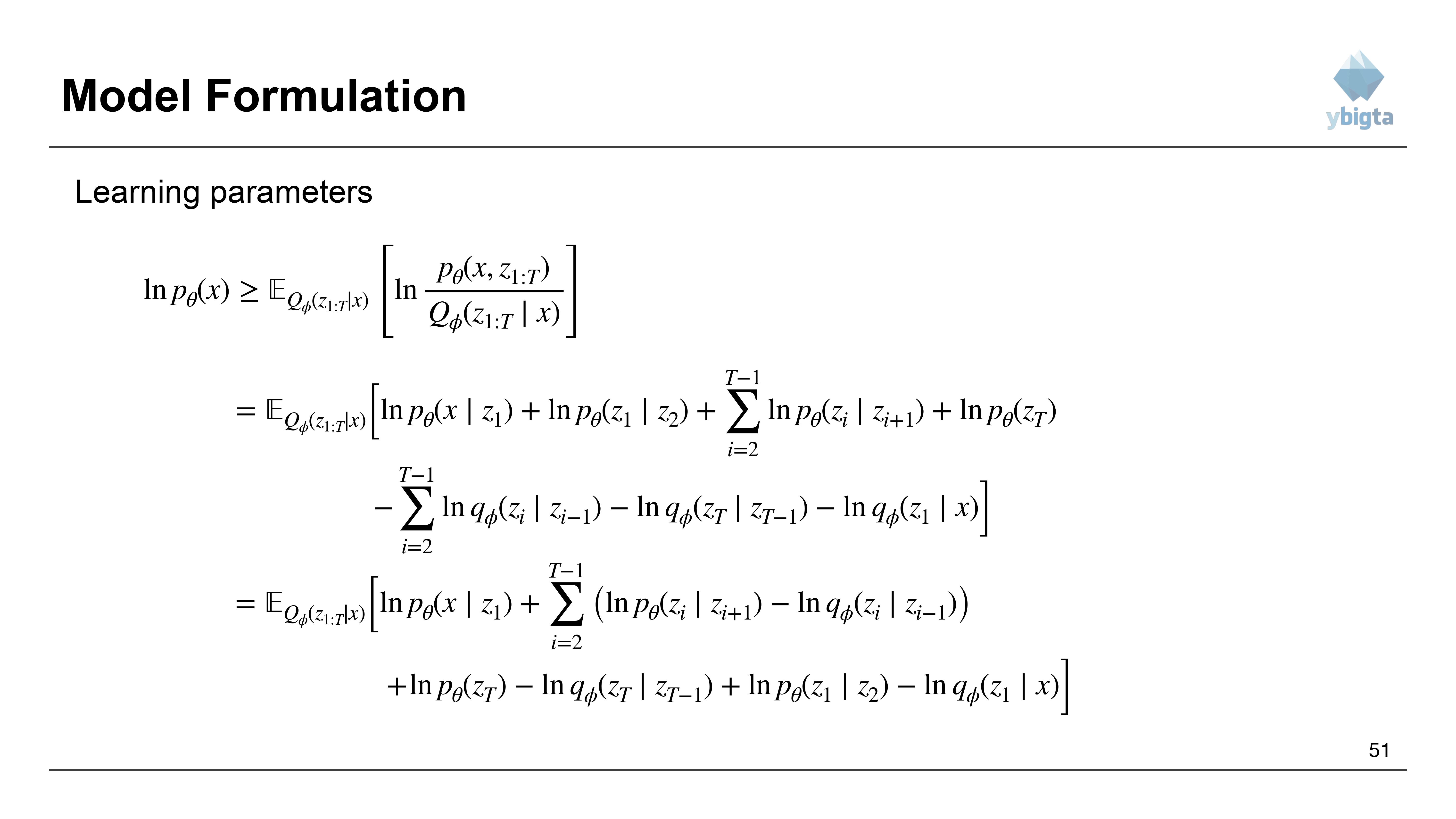
- Grouping terms: $$= E_{Q_{\phi}} [\ln p_{\theta}(x|z_1) + \ln p_{\theta}(z_1|z_2) + \sum_{i=2}^{T-1} \ln p_{\theta}(z_i|z_{i+1}) + \ln p_{\theta}(z_T)$$ $$- \sum_{i=2}^{T-1} \ln q_{\phi}(z_i|z_{i-1}) - \ln q_{\phi}(z_T|z_{T-1}) - \ln q_{\phi}(z_1|x)]$$
Slide 51: Regrouping for KL Divergence
- We want to pair matching $p$ and $q$ terms to form KL Divergences.
- Grouping $(p_{\theta}(z_i|z_{i+1})$ and $q_{\phi}(z_i|z_{i-1}))$.
Slide 52: KL Divergence Recap
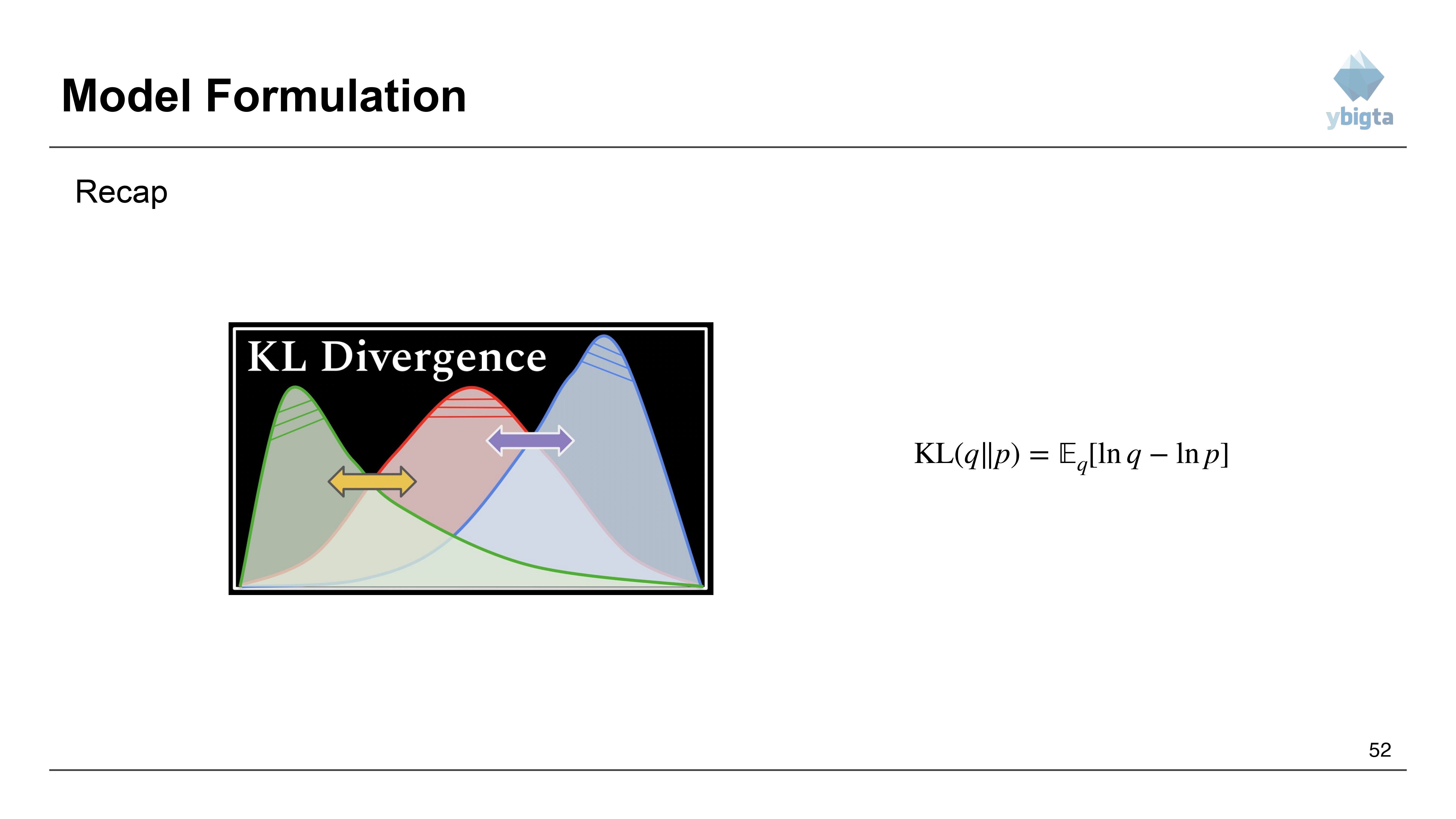
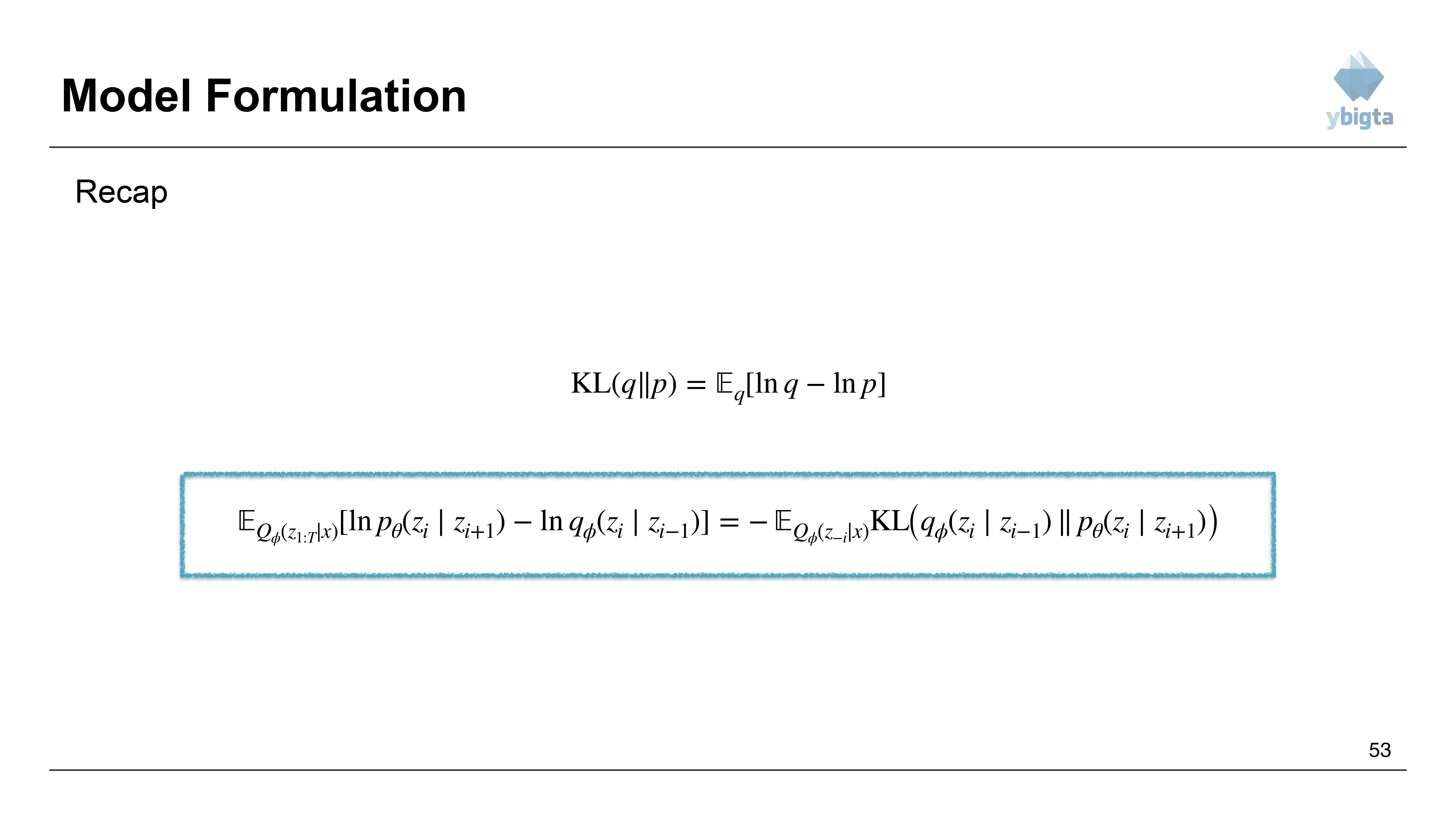
- Definition: $KL(q||p) = \mathbb{E}_q [\ln q - \ln p]$
- We will use this to simplify the expectation terms.
Slide 53: Applying KL Definition
- $E_{Q_{\phi}} [\ln p - \ln q] = - E_{Q_{\phi}} [\ln q - \ln p] = - KL(q||p)$
Slide 54: Identifying Terms (1)
- Looking at the expanded equation again to match terms.
Slide 55: Identifying Terms (2)
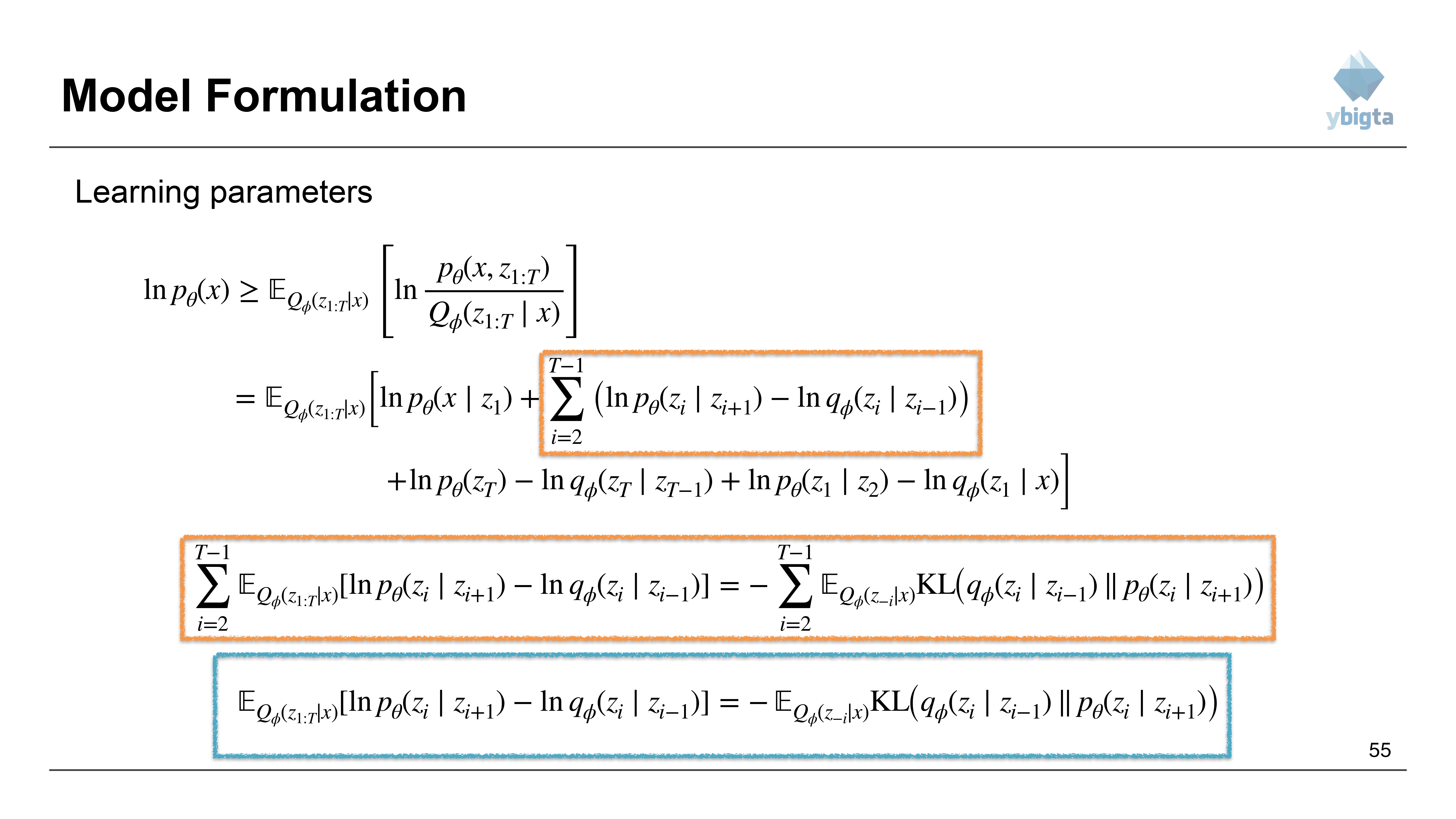
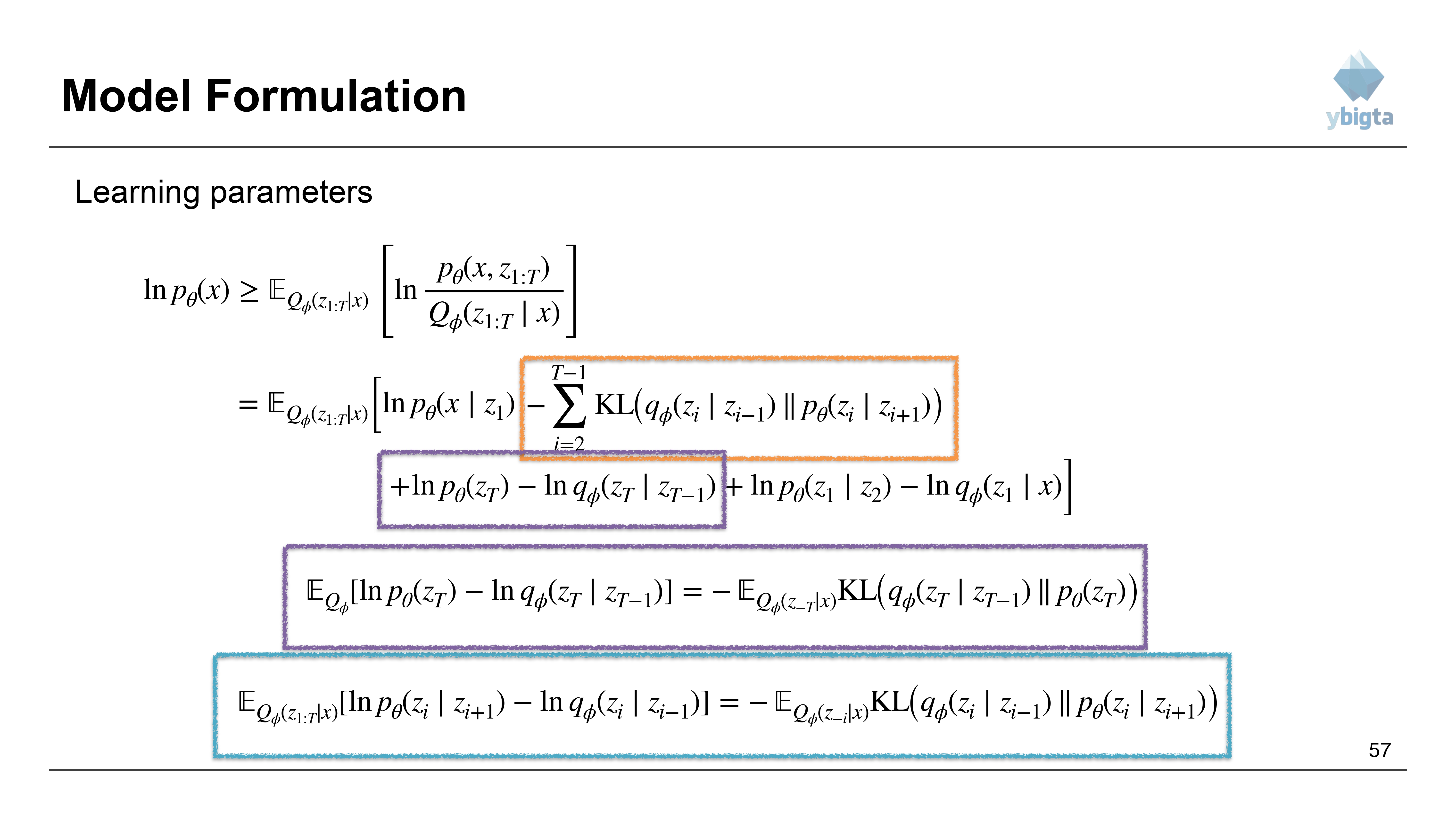
- The sum term becomes a sum of KL divergences: $$\sum_{i=2}^{T-1} E [\ln p_{\theta}(z_i|z_{i+1}) - \ln q_{\phi}(z_i|z_{i-1})] = - \sum_{i=2}^{T-1} KL(q_{\phi}(z_i|z_{i-1}) || p_{\theta}(z_i|z_{i+1}))$$
Slide 56: Identifying Terms (3)
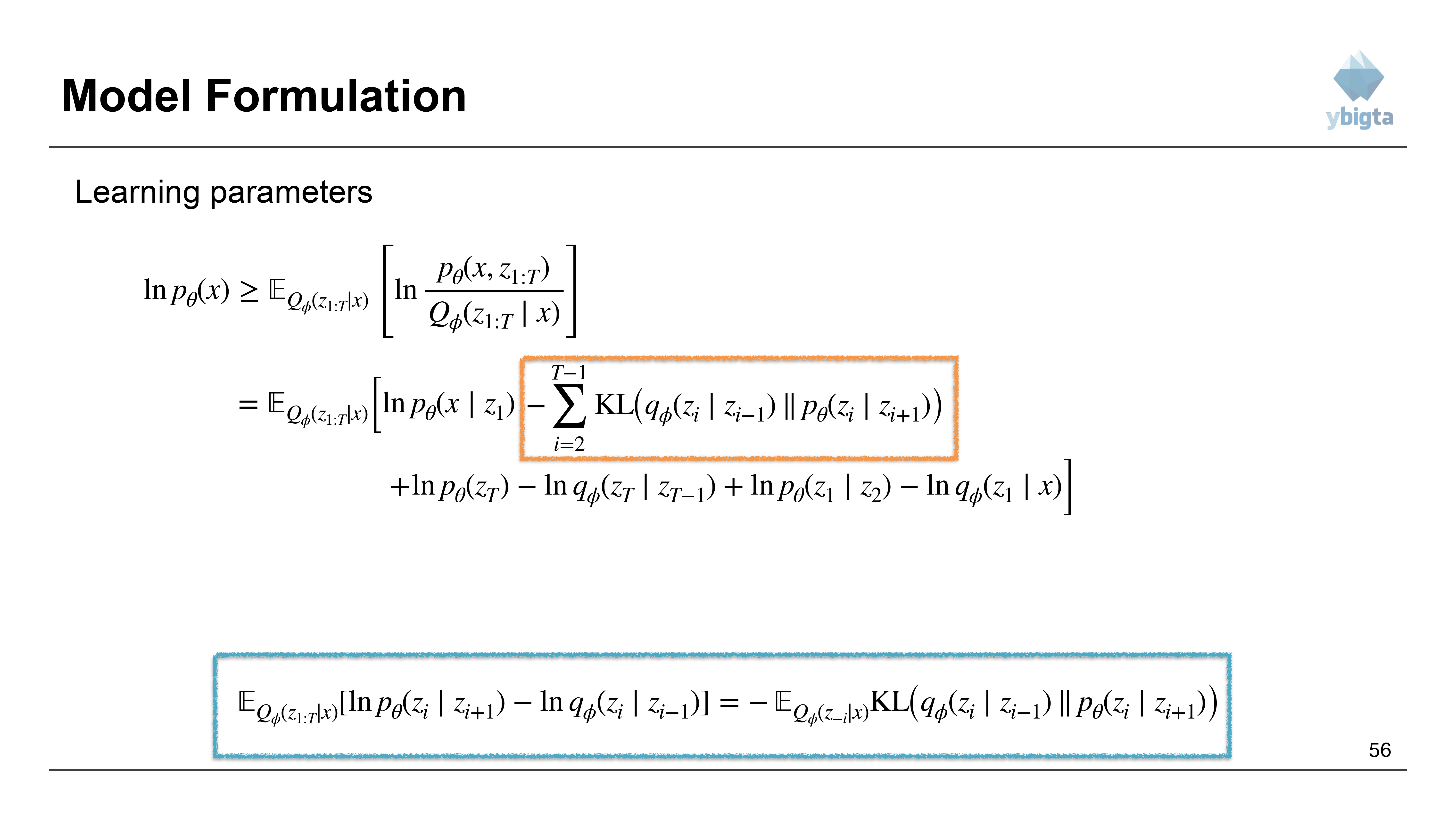
- Placing the summation term back into the equation.
Slide 57: Identifying Terms (4)
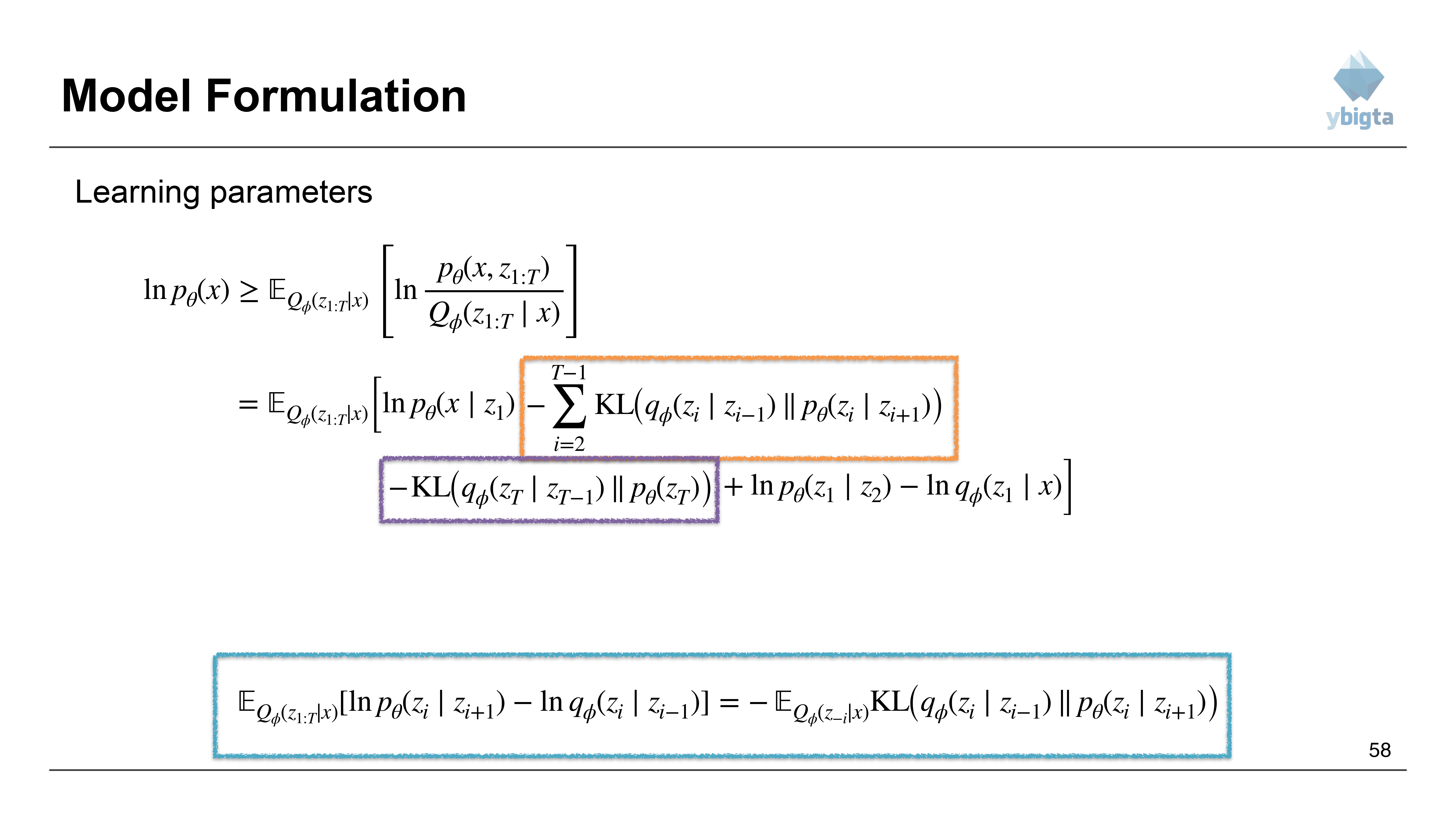
- Dealing with the $z_T$ term: $$E [\ln p_{\theta}(z_T) - \ln q_{\phi}(z_T|z_{T-1})] = - KL(q_{\phi}(z_T|z_{T-1}) || p_{\theta}(z_T))$$
Slide 58: Identifying Terms (5)
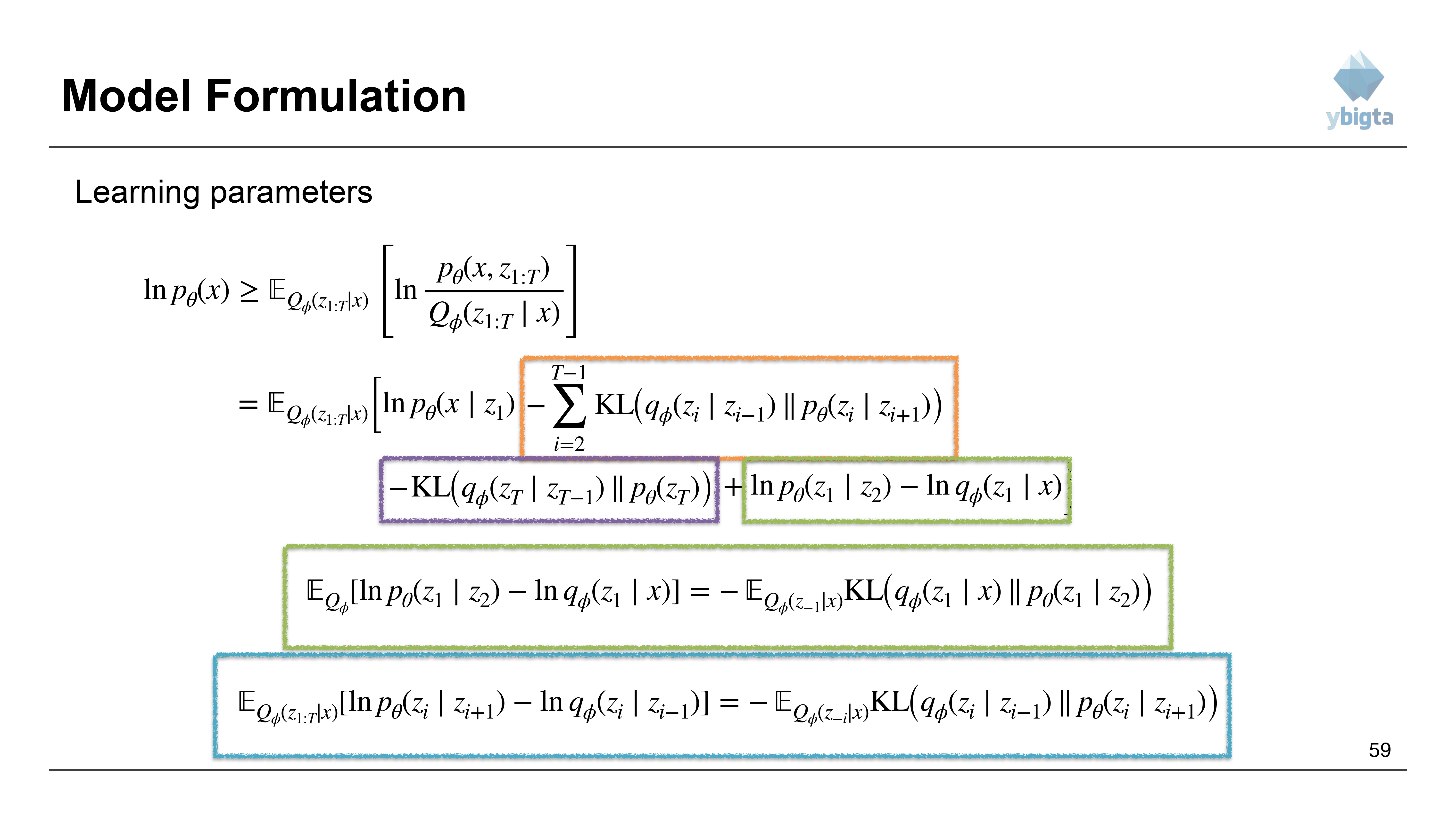
- Only the $z_1$ term and reconstruction term remain.
Slide 59: Identifying Terms (6)
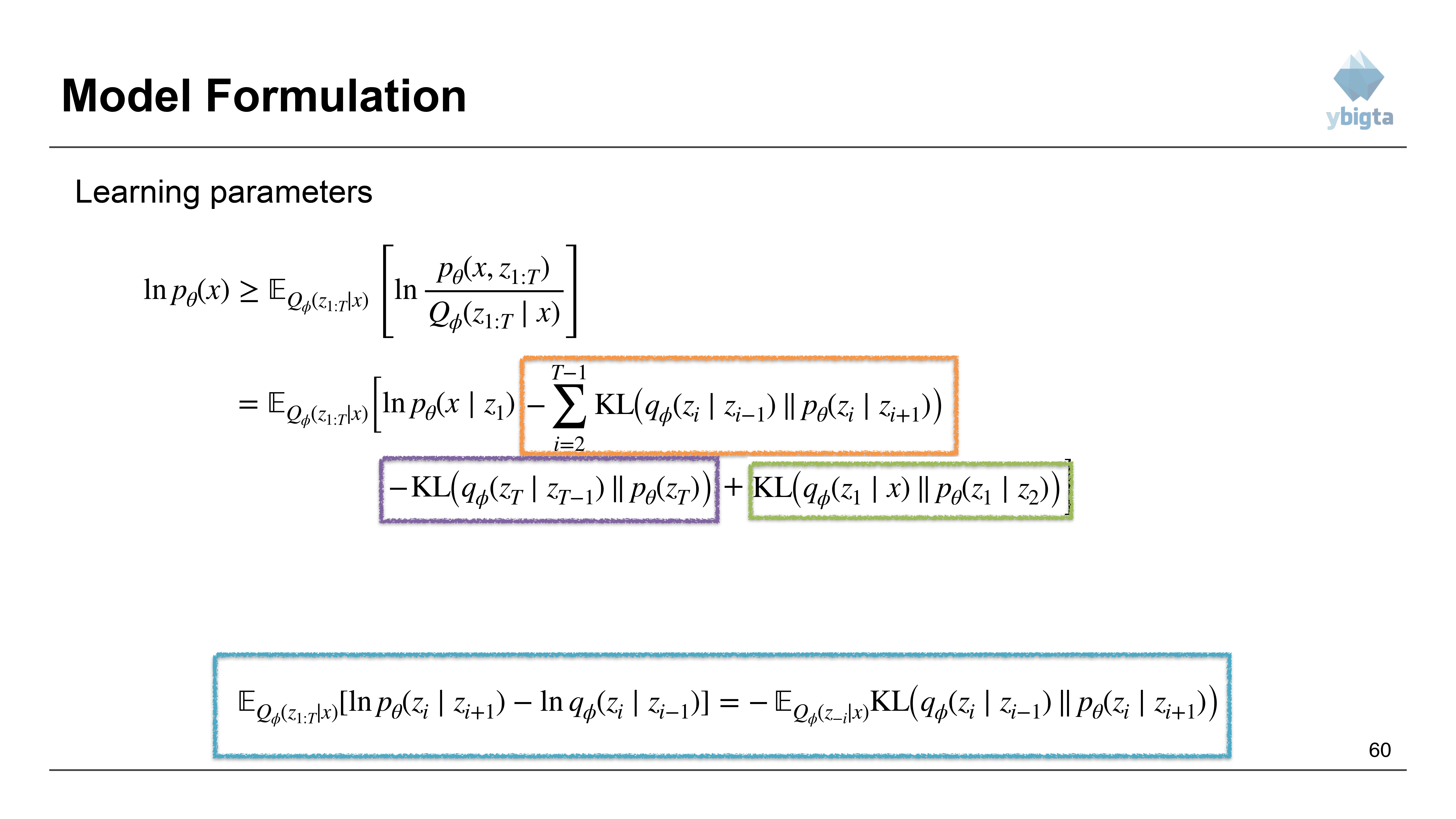
- The $z_1$ term: $$E [\ln p_{\theta}(z_1|z_2) - \ln q_{\phi}(z_1|x)] = - KL(q_{\phi}(z_1|x) || p_{\theta}(z_1|z_2))$$
Slide 60: Final Grouping
- All terms are now converted to Expectations or KL divergences.
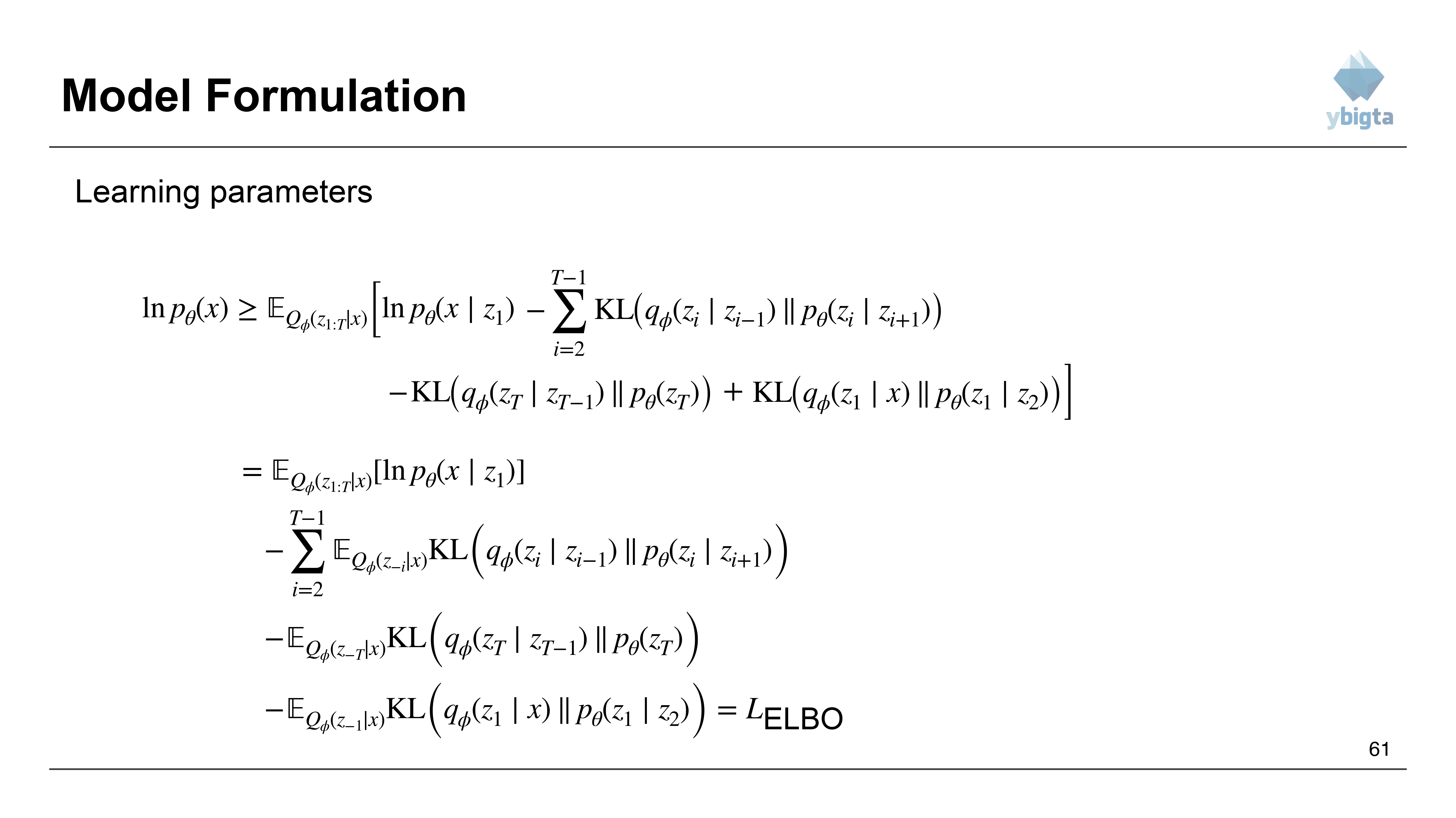
Slide 61: The ELBO Equation
- Evidence Lower Bound (ELBO):
$$
\begin{aligned}
L_{ELBO} &= \mathbb{E}_{Q_{\phi}} [\ln p_{\theta}(x|z_1)] \\
&\quad - \sum_{i=2}^{T-1} KL\big(q_{\phi}(z_i \mid z_{i-1}) \,\|\, p_{\theta}(z_i \mid z_{i+1})\big) \\
&\quad - KL\big(q_{\phi}(z_T \mid z_{T-1}) \,\|\, p_{\theta}(z_T)\big) \\
&\quad - KL\big(q_{\phi}(z_1 \mid x) \,\|\, p_{\theta}(z_1 \mid z_2)\big)
\end{aligned}
$$
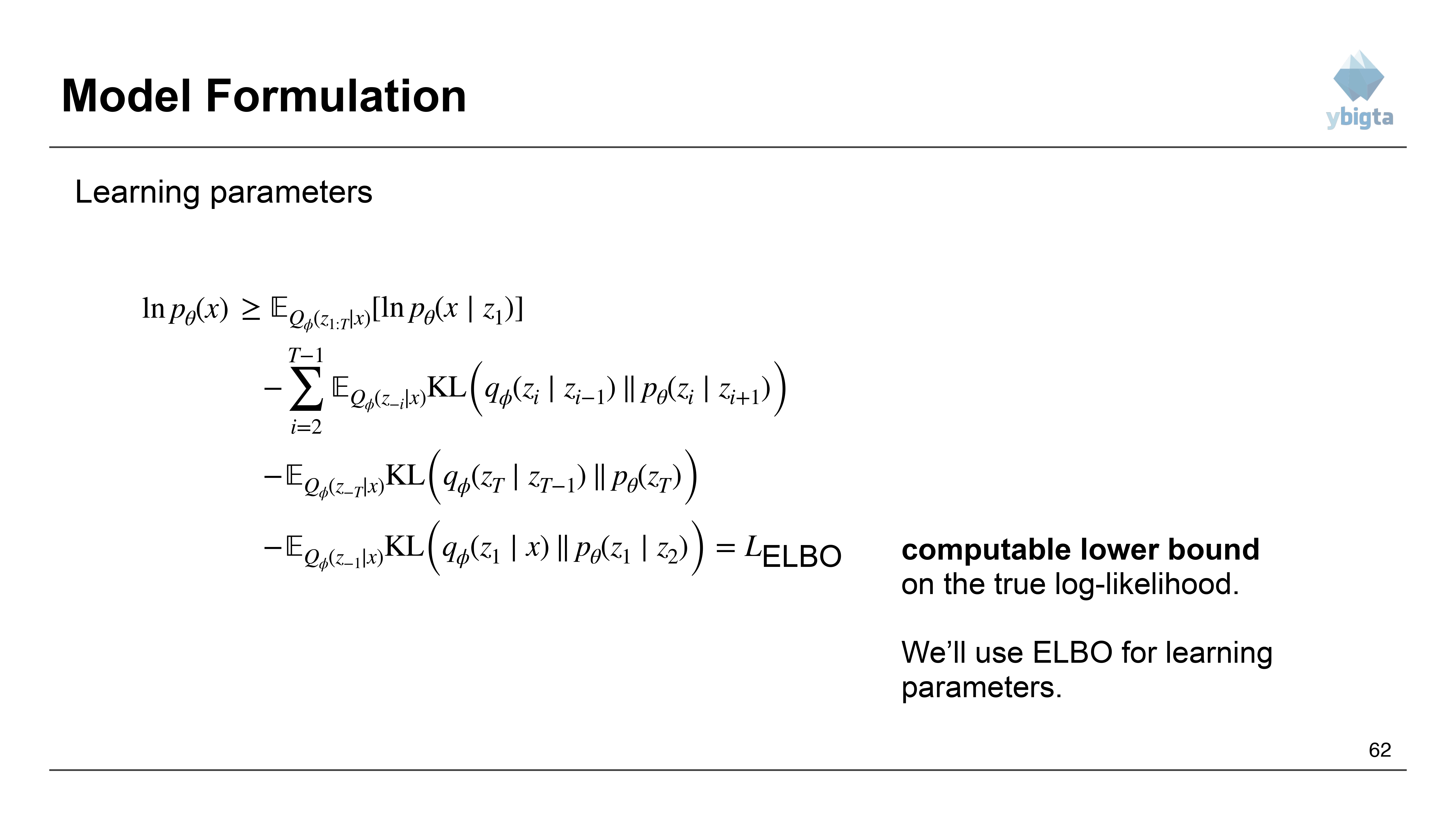
Slide 62: Usefulness of ELBO
- This gives us a computable lower bound on the true log-likelihood.
- We maximize this ELBO to learn the parameters.
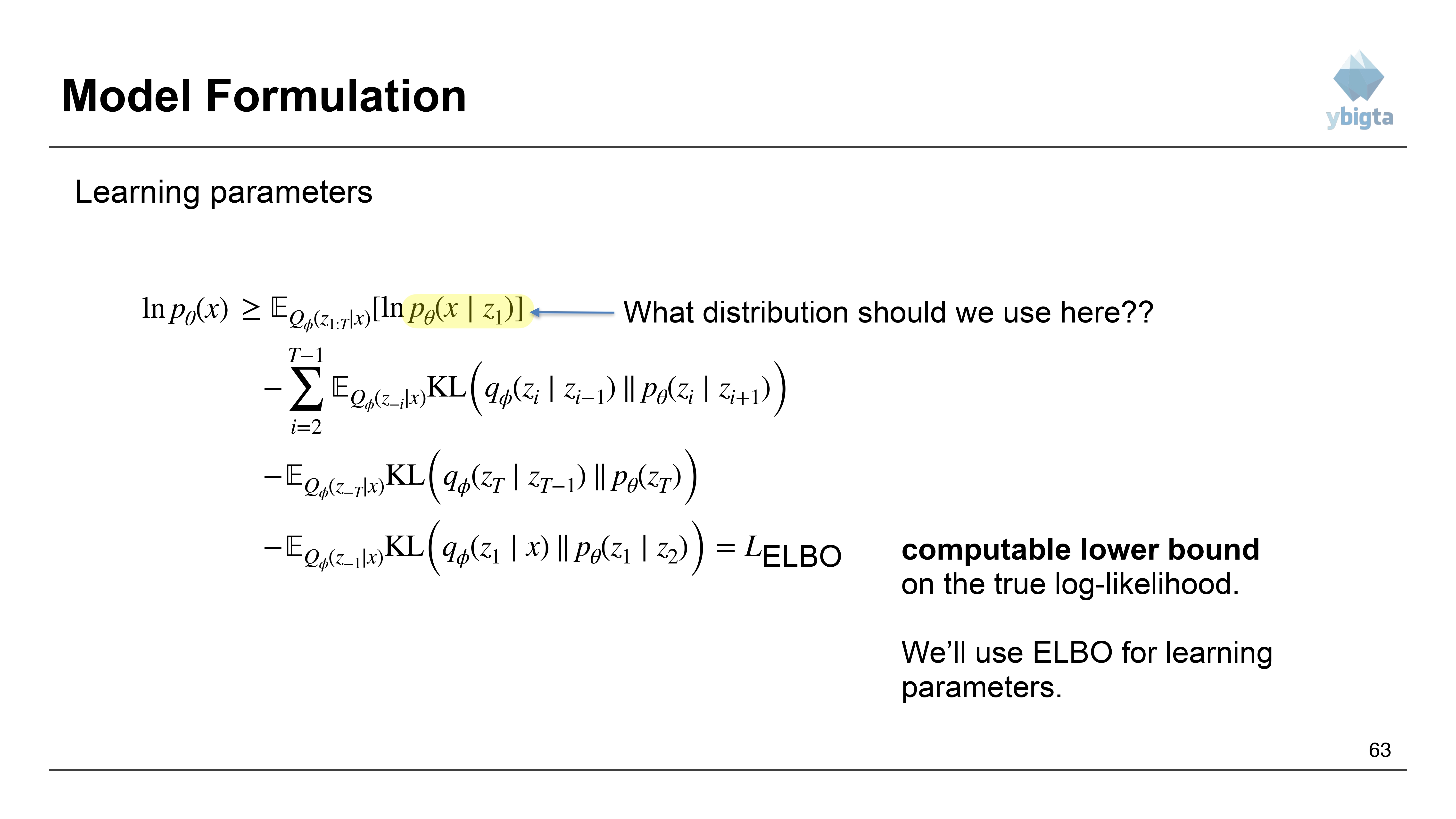
Slide 63: The Reconstruction Term
- Focus on the first term: $\mathbb{E}{Q{\phi}} [\ln p_{\theta}(x|z_1)]$
- What distribution should we use for $p_{\theta}(x|z_1)$?
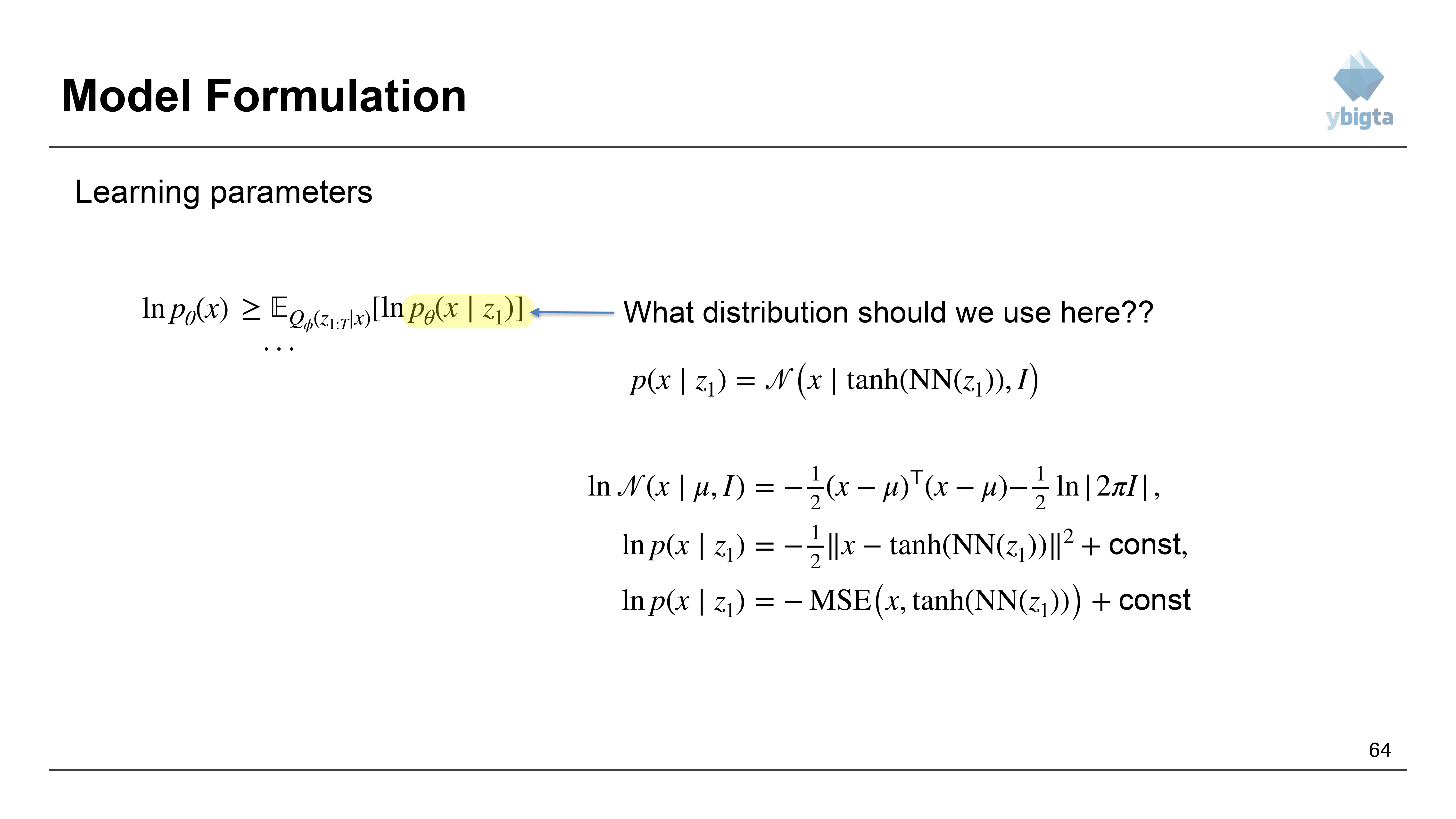
Slide 64: Gaussian Reconstruction
- Assume Gaussian distribution: $p(x|z_1) = \mathcal{N}(x | \tanh(NN(z_1)), I)$
- The log-likelihood of a Gaussian is proportional to the negative Mean Squared Error (MSE).
- $\ln p(x|z_1) = -MSE(x, \tanh(NN(z_1))) + const$
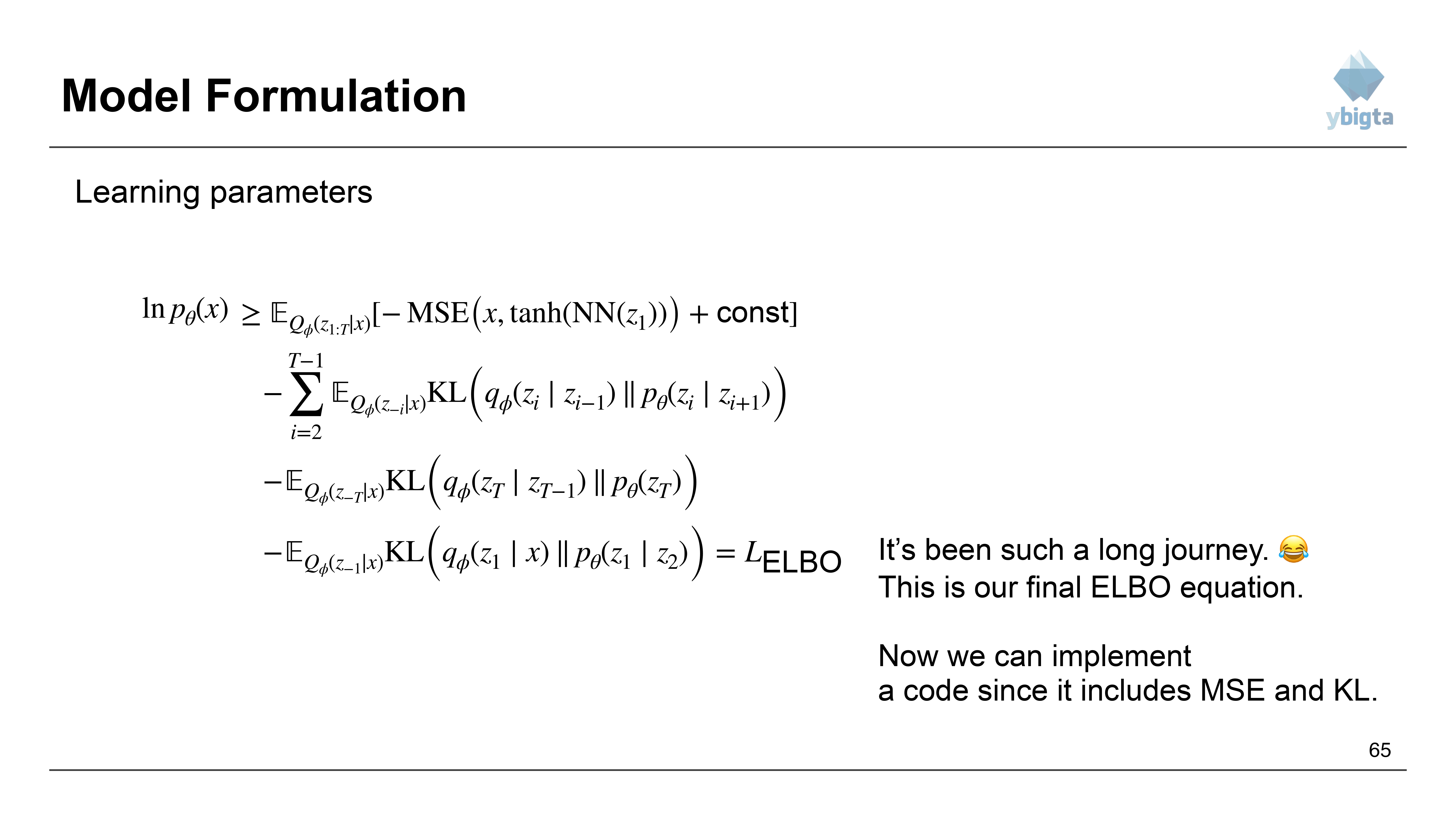
Slide 65: Final ELBO for Implementation
- Result: $$L_{ELBO} = E[-MSE] - \sum KL - KL - KL$$
- Now we can implement this in code since it consists of MSE and KL divergence terms, which are differentiable.
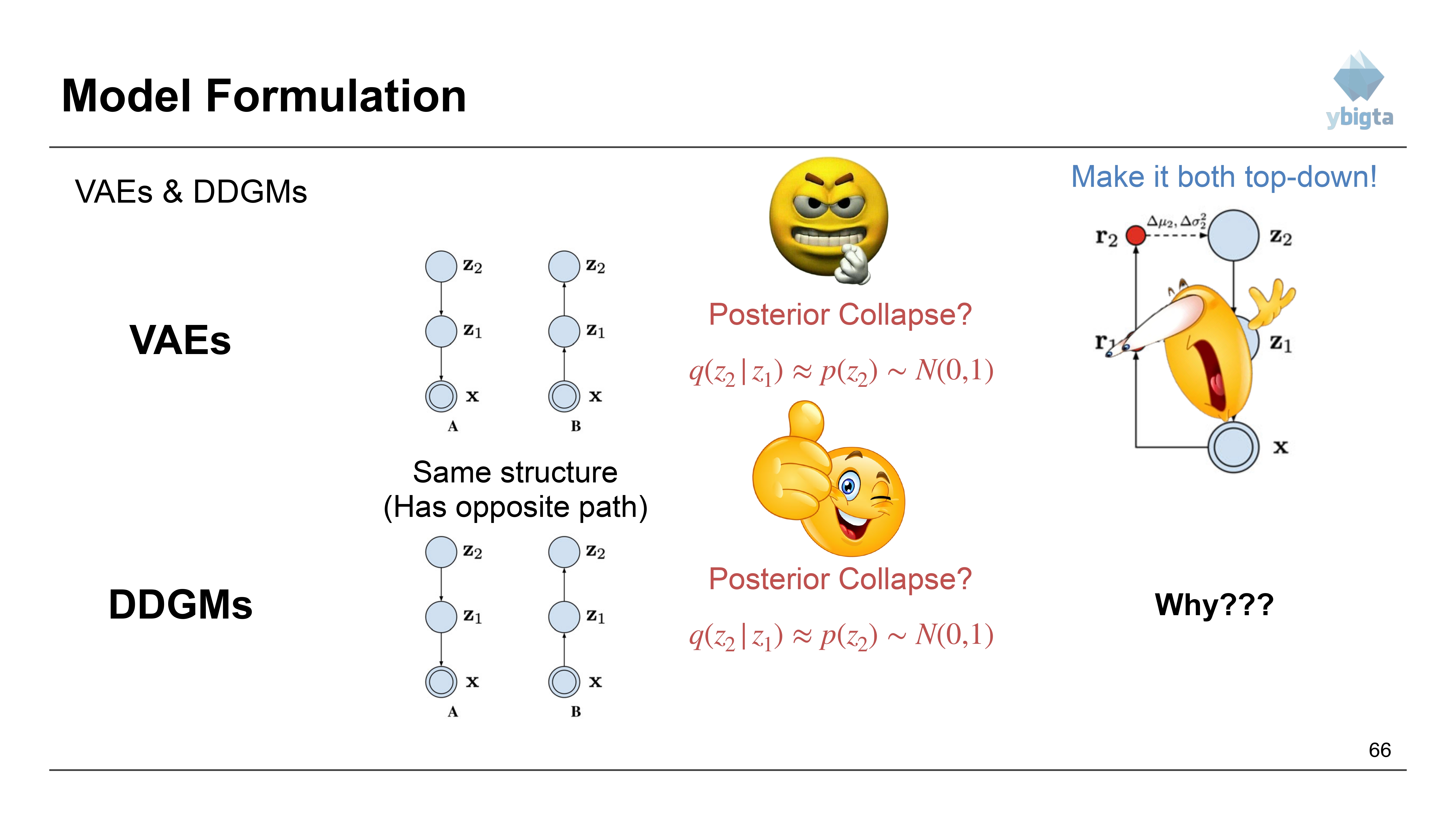
Slide 66: Revisiting the VAE Comparison
- Why did we go through all this math? To check stability and Posterior Collapse again.
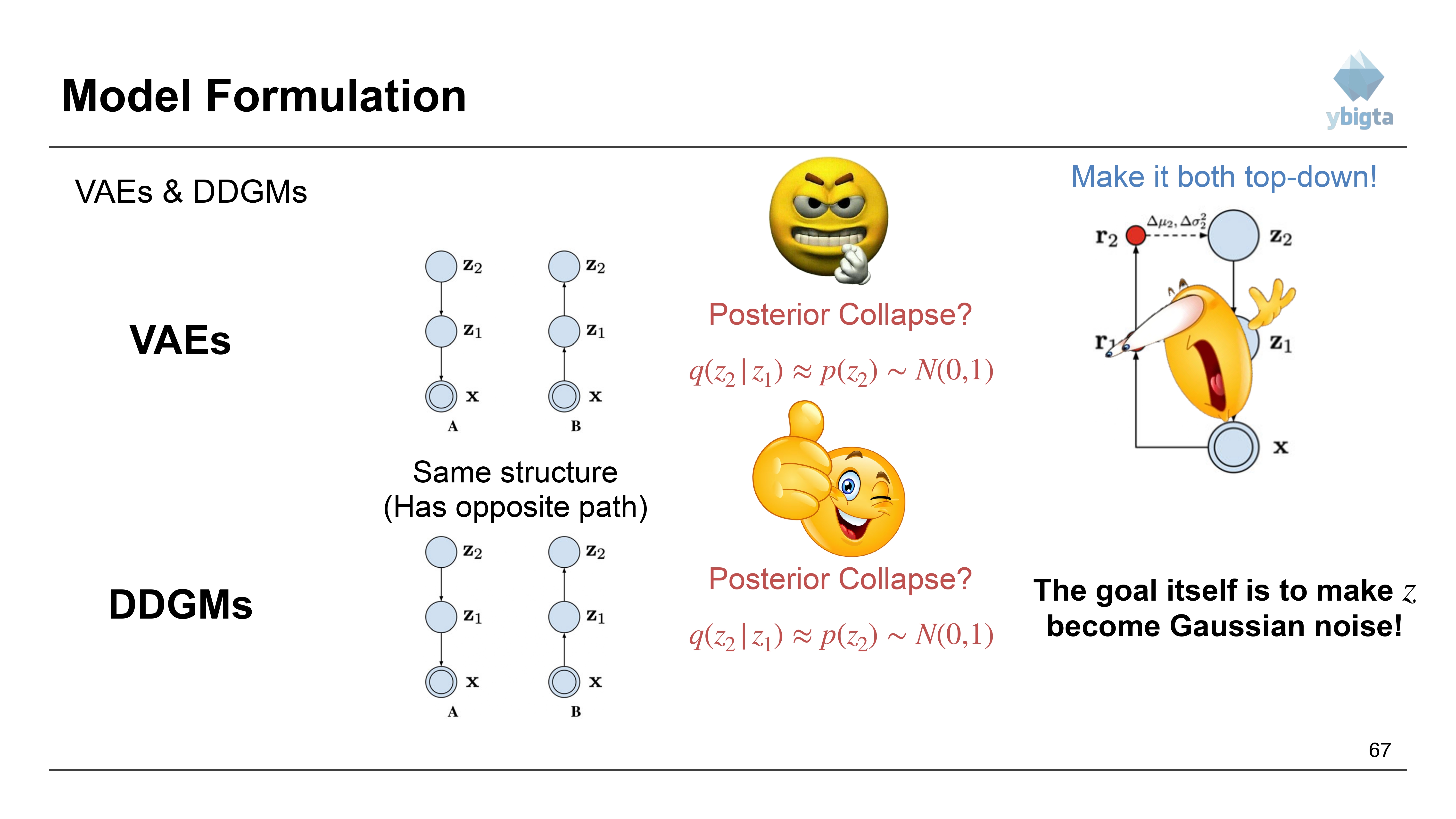
Slide 67: Posterior Collapse in DDGMs?
- VAE: Collapsed if $q(z|x) \approx \mathcal{N}(0,1)$.
- DDGM: The goal is to make $z$ become Gaussian noise!
- So “collapse” in the VAE sense is actually the objective of the forward diffusion process.
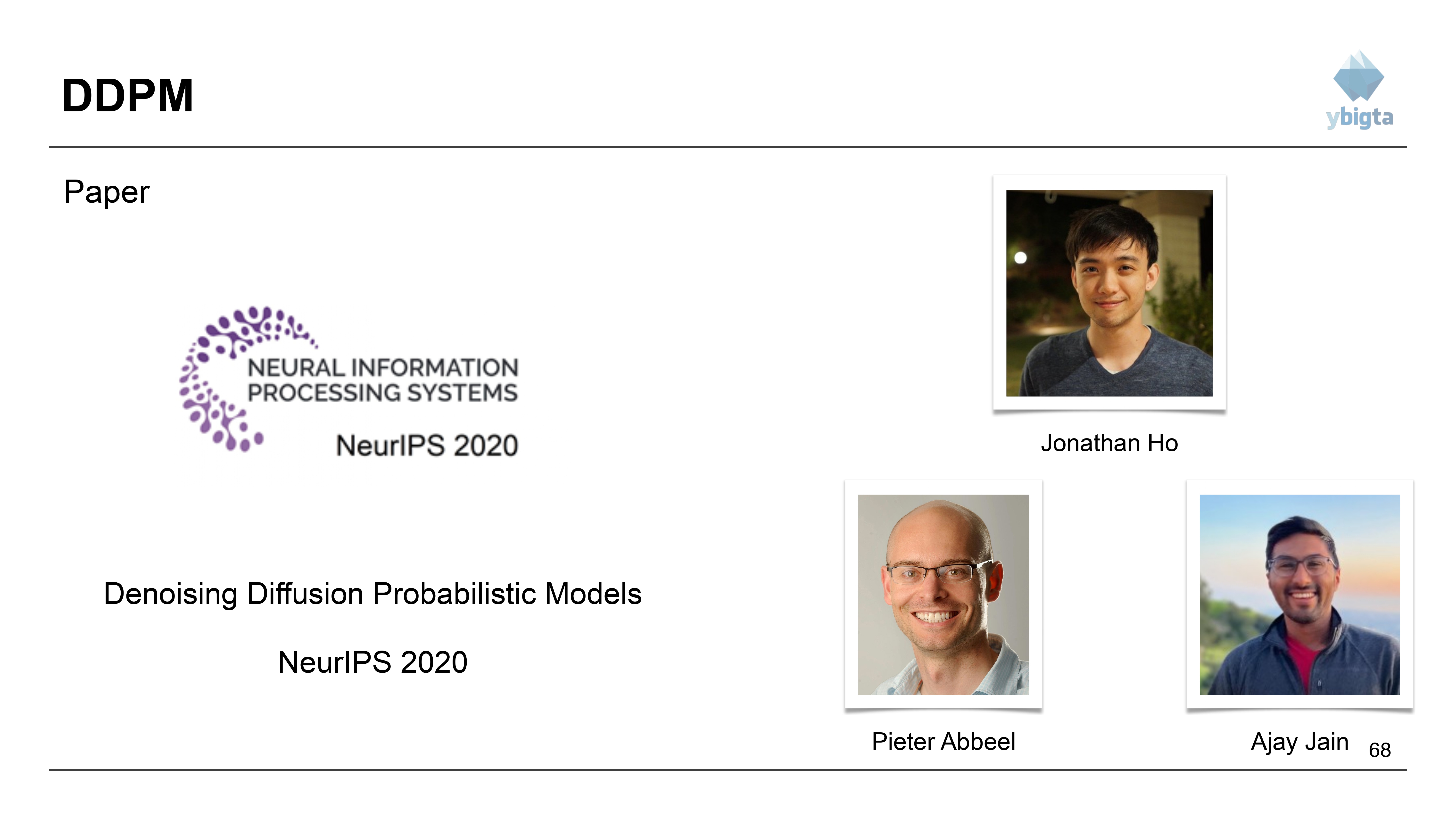
Slide 68: DDPM Paper
- Paper: Denoising Diffusion Probabilistic Models (NeurIPS 2020).
- Authors: Jonathan Ho, Ajay Jain, Pieter Abbeel.
- This paper simplified the training of diffusion models significantly.
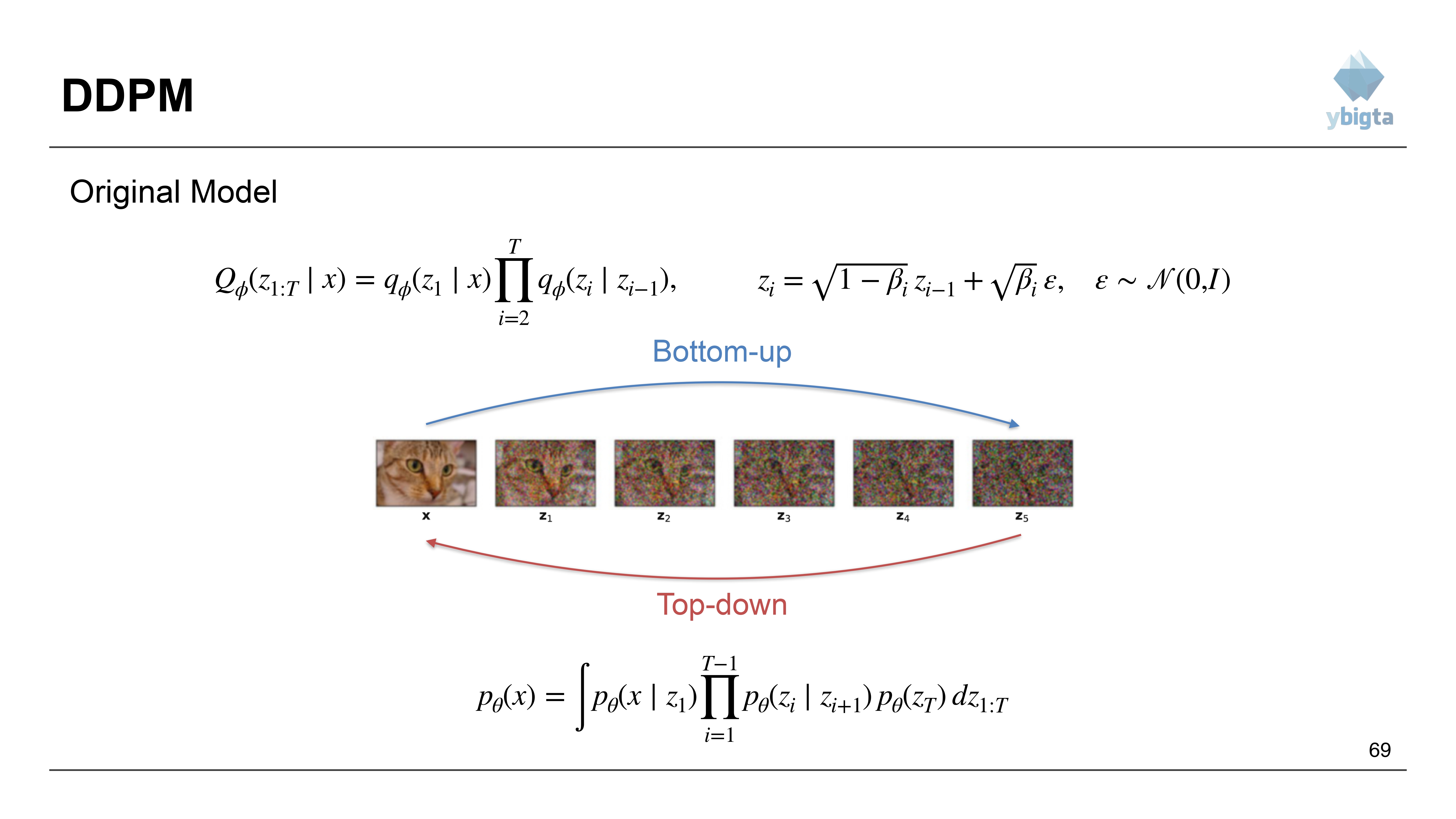
Slide 69: Original Model Recap
- Bottom-up (Forward): Gaussian noise steps.
- Top-down (Reverse): Learned denoising.
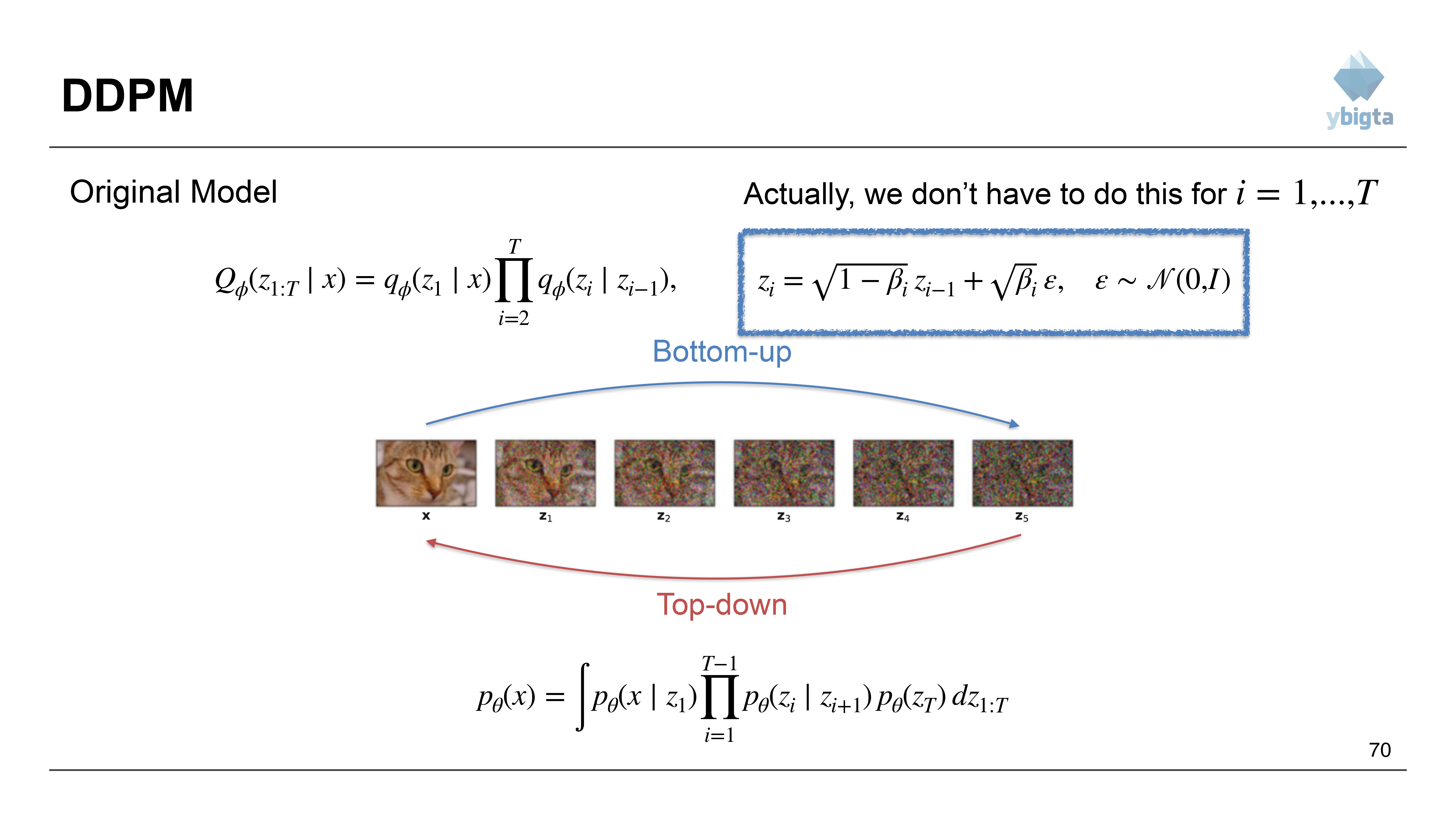
Slide 70: Efficiency Problem
- Do we have to sample iteratively $i=1…T$ just to get the forward noise $z_T$?
- $z_i = \sqrt{1-\beta_i}z_{i-1} + \sqrt{\beta_i}\epsilon$
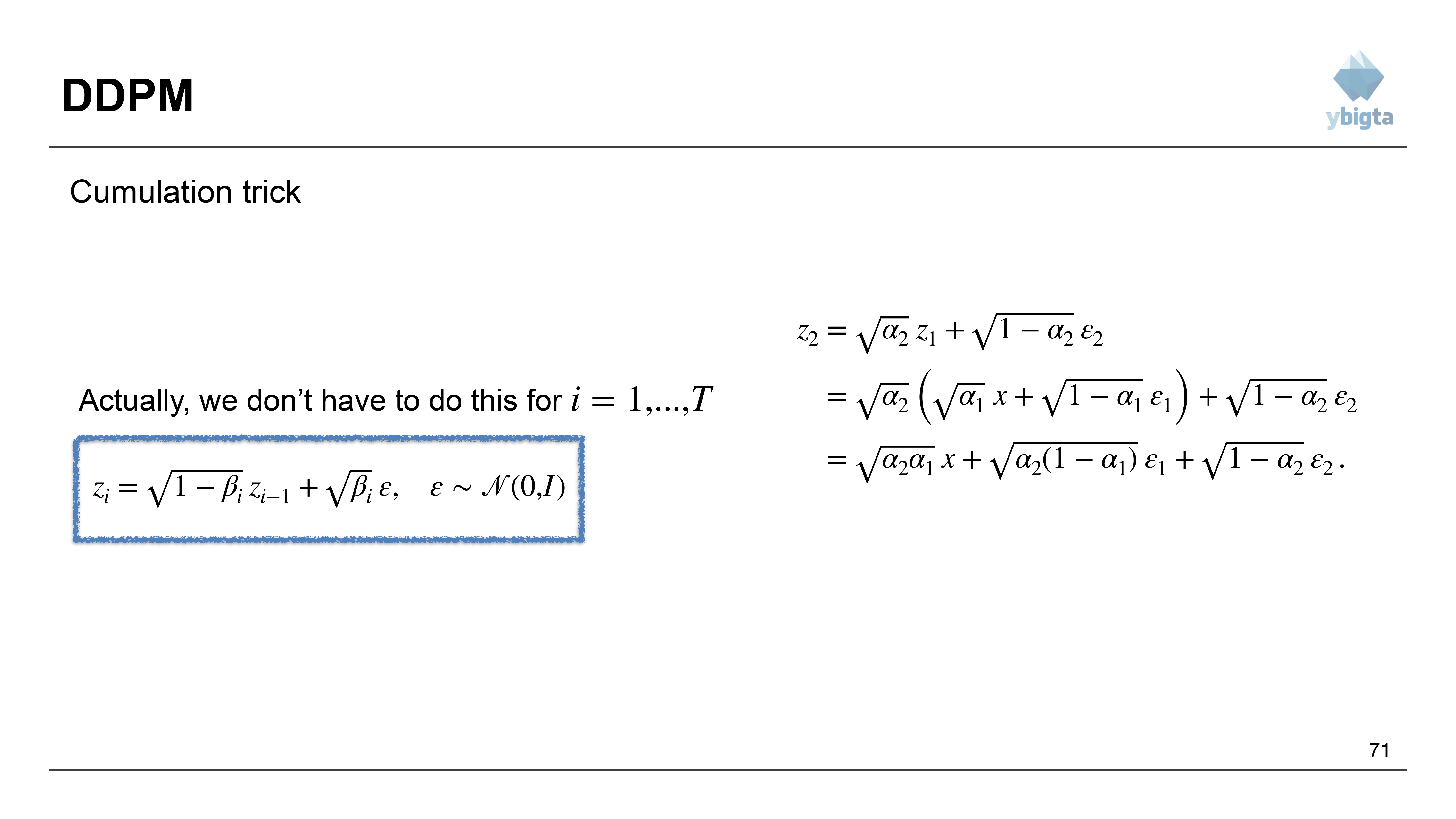
Slide 71: Cumulation Trick (1)
- We can skip steps.
- $z_2 = \sqrt{\alpha_2}z_1 + \sqrt{1-\alpha_2}\epsilon_2$
- Substitute $z_1$: $z_2 = \sqrt{\alpha_2}(\sqrt{\alpha_1}x + \sqrt{1-\alpha_1}\epsilon_1) + \sqrt{1-\alpha_2}\epsilon_2$ (Where $\alpha_i = 1 - \beta_i$)
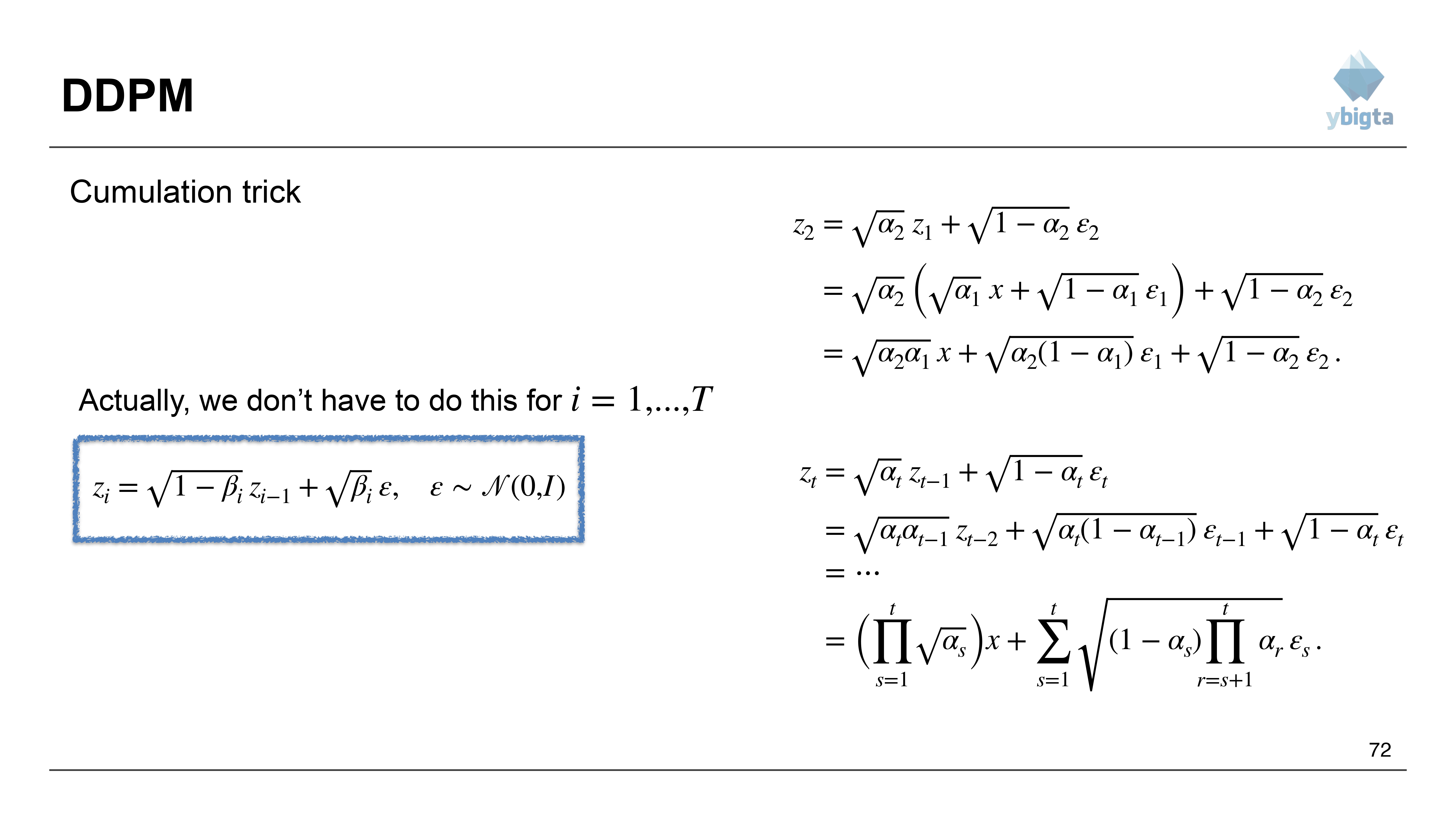
Slide 72: Cumulation Trick (2)
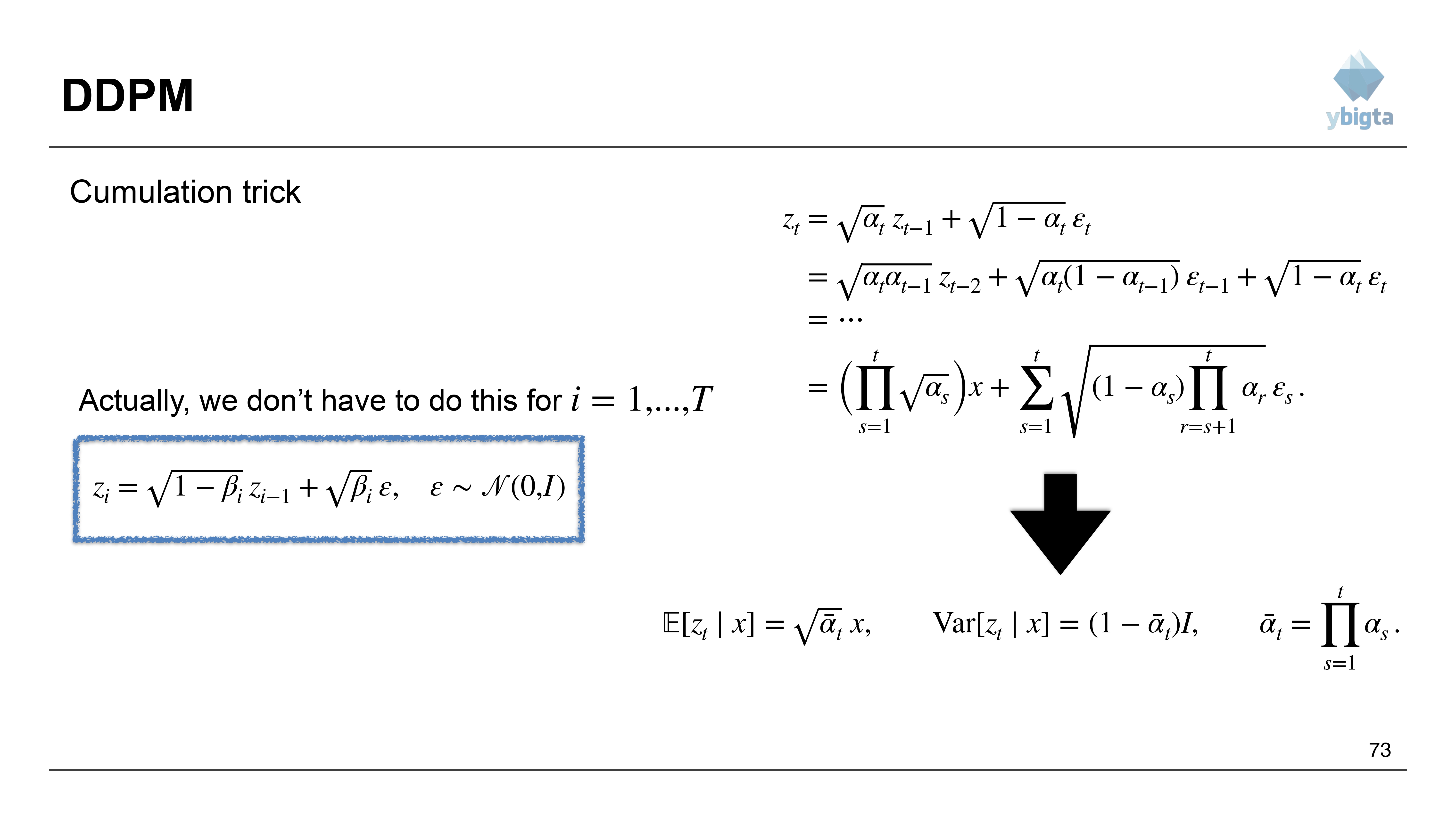
- Combining Gaussians: $z_t = \sqrt{\alpha_t}z_{t-1} + \sqrt{1-\alpha_t}\epsilon_t$
- By induction, we can express $z_t$ directly from $x$.
Slide 73: Cumulation Trick (3)
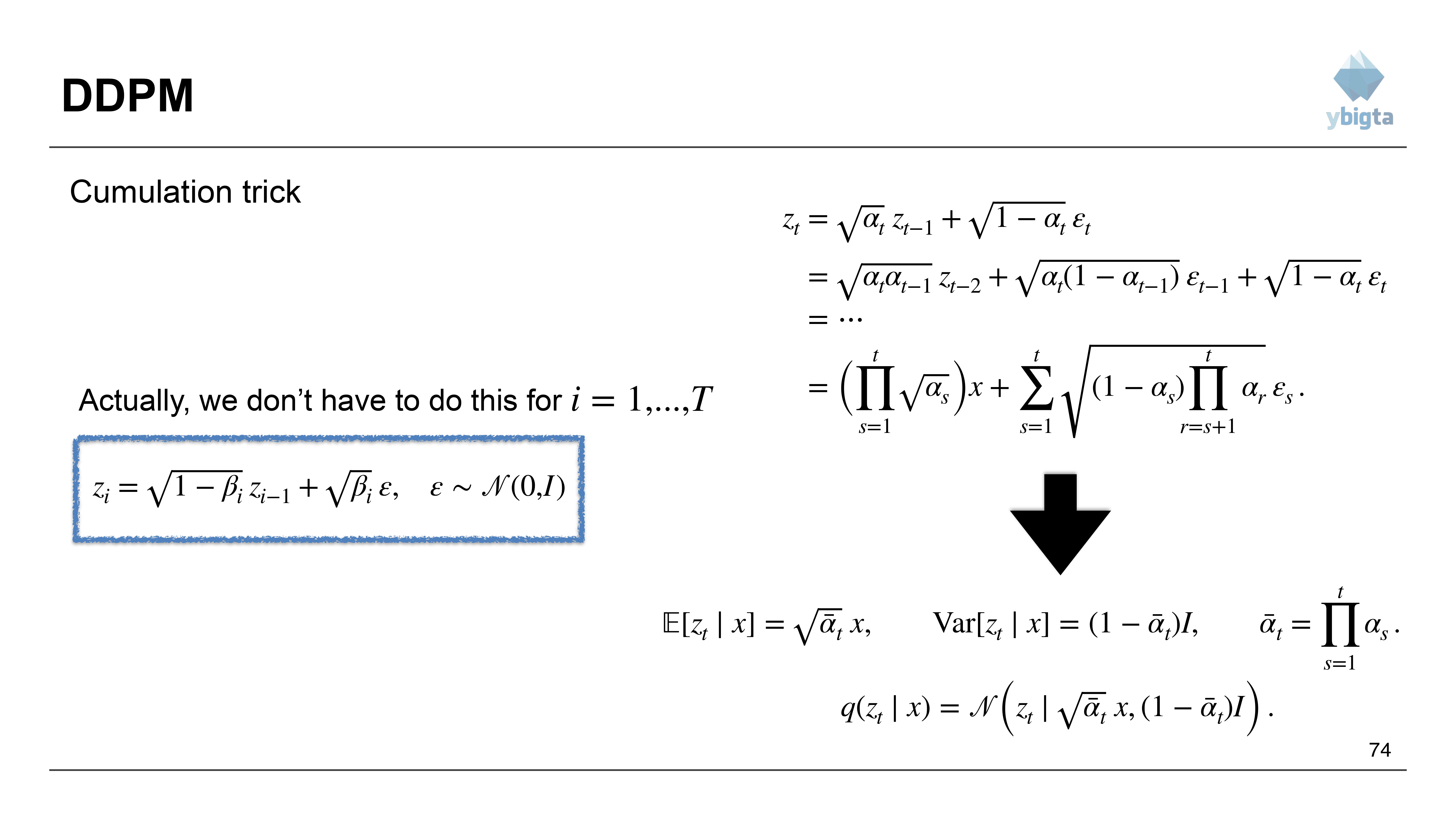
- Result: $$z_t = \sqrt{\bar{\alpha}_t}x + \sqrt{1-\bar{\alpha}_t}\epsilon$$
- Where $\bar{\alpha}t = \prod{s=1}^t \alpha_s$.
- Mean: $\sqrt{\bar{\alpha}_t}x$
- Variance: $(1-\bar{\alpha}_t)I$
Slide 74: Closed Form Forward Step
- We can sample $z_t$ at any timestep $t$ in one go: $$q(z_t|x) = \mathcal{N}(z_t | \sqrt{\bar{\alpha}_t}x, (1-\bar{\alpha}_t)I)$$
Slide 75: New Model Formulation
- Forward: Directly sample $z_t$ using the cumulation trick.
- Reverse: Same learned process.
Slide 76: DDPM Learning Parameters
- We revisit the loss function derivation with this new trick in mind.
- Objective: Maximize $\ln p_{\theta}(x)$.
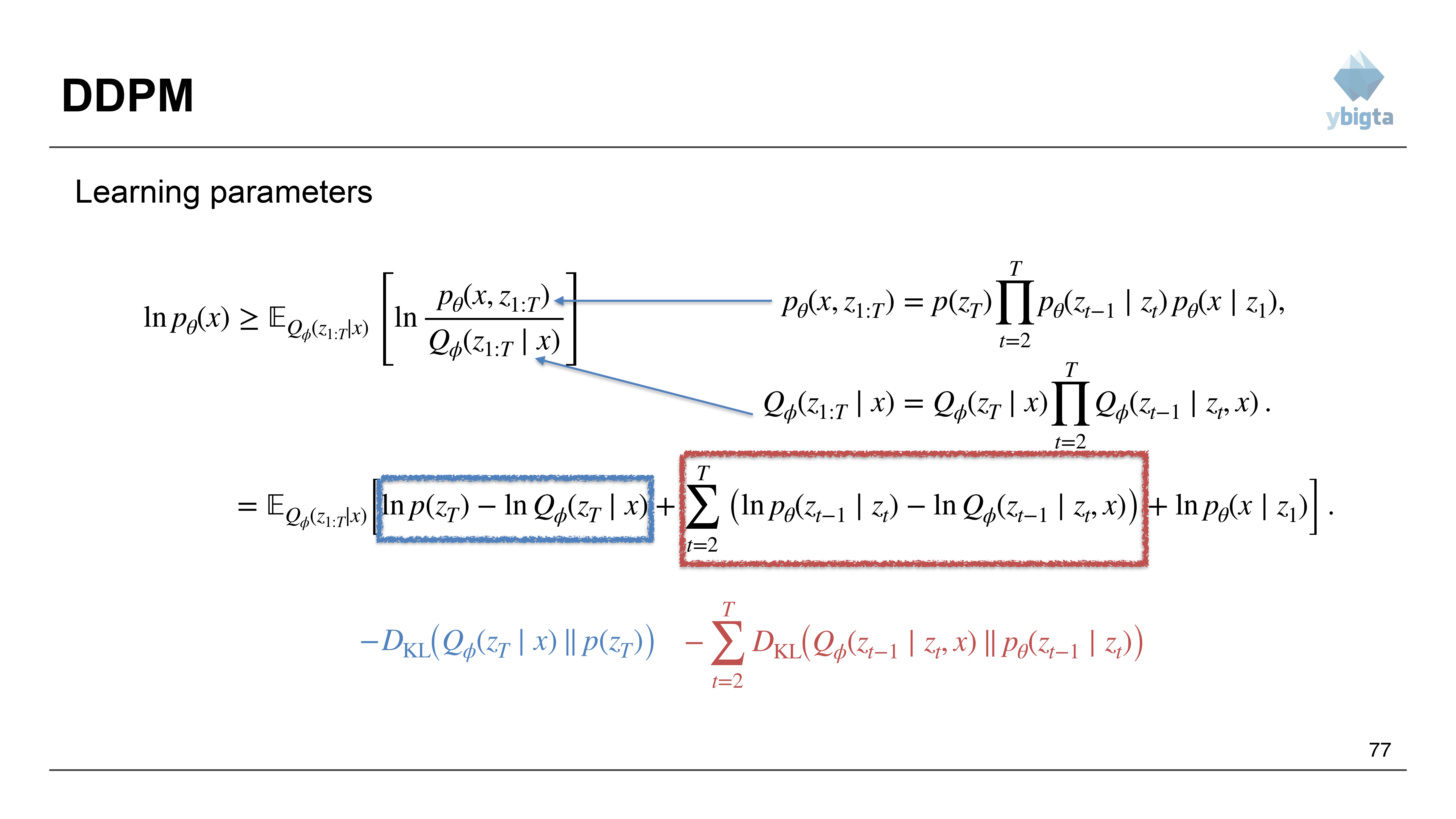
Slide 77: Deriving DDPM Loss (1)
- Using the same variational bound logic: $$= E_Q [\ln \frac{p(z_T) \prod p(z_{t-1}|z_t) p(x|z_1)}{Q(z_T|x) \prod Q(z_{t-1}|z_t, x)}]$$
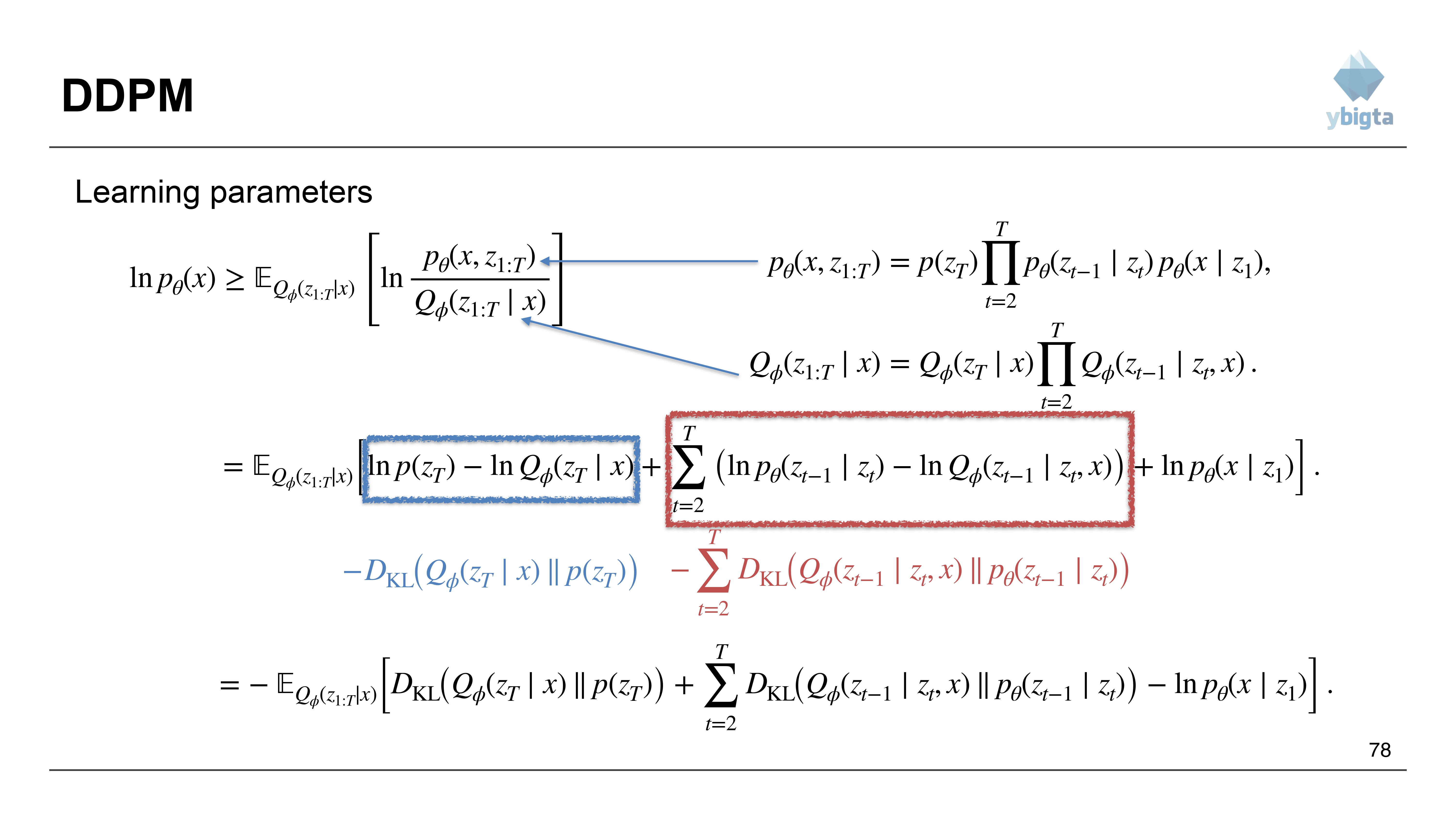
Slide 78: Deriving DDPM Loss (2)
- Grouping terms into KL divergences again.
- Terminology:
- $L_T$: KL between $Q(z_T|x)$ and $p(z_T)$ (Prior matching).
- $L_{t-1}$: KL between $Q(z_{t-1}|z_t, x)$ and $p_{\theta}(z_{t-1}|z_t)$ (Denoising matching).
- $L_0$: Reconstruction log likelihood.
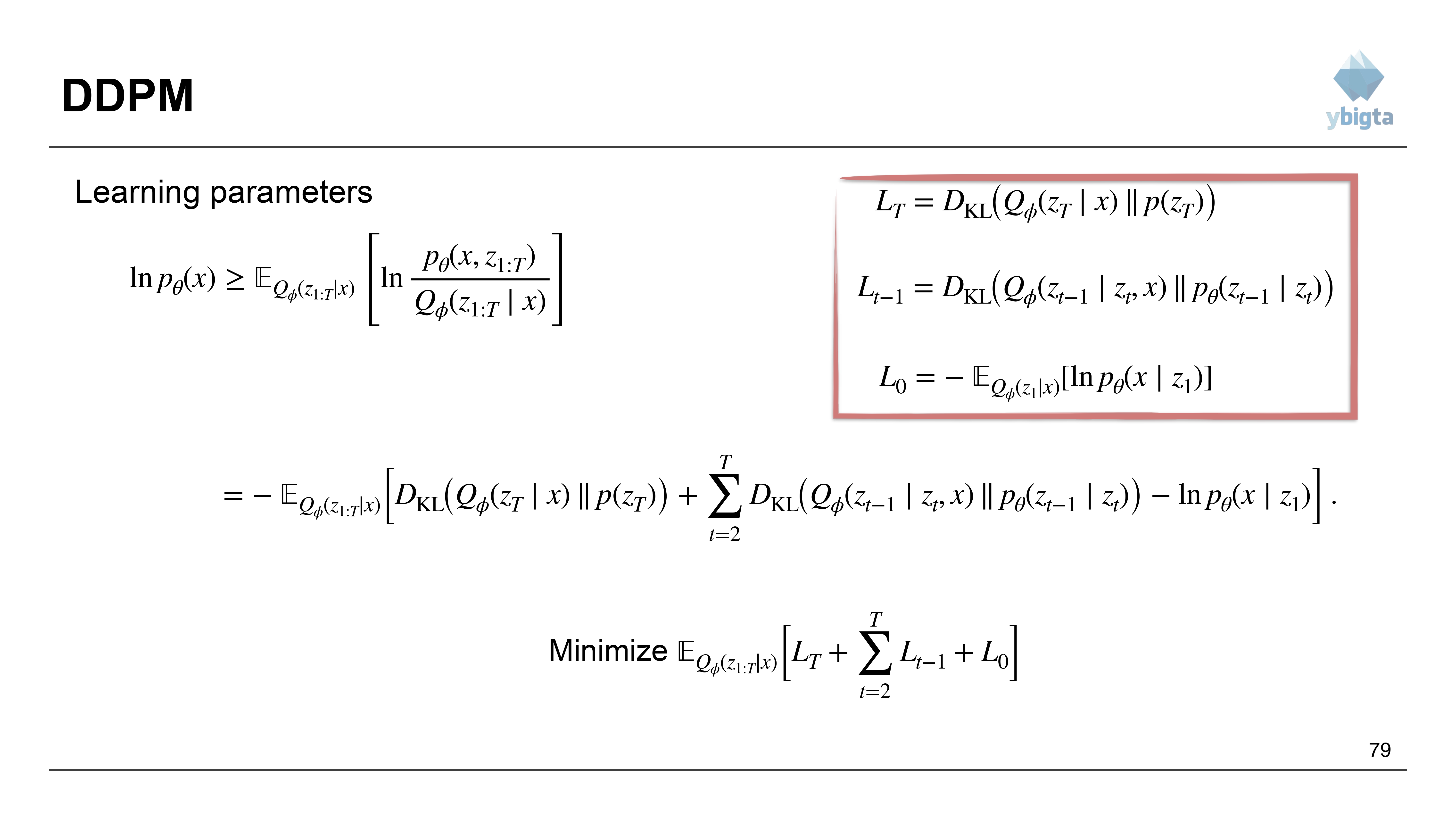
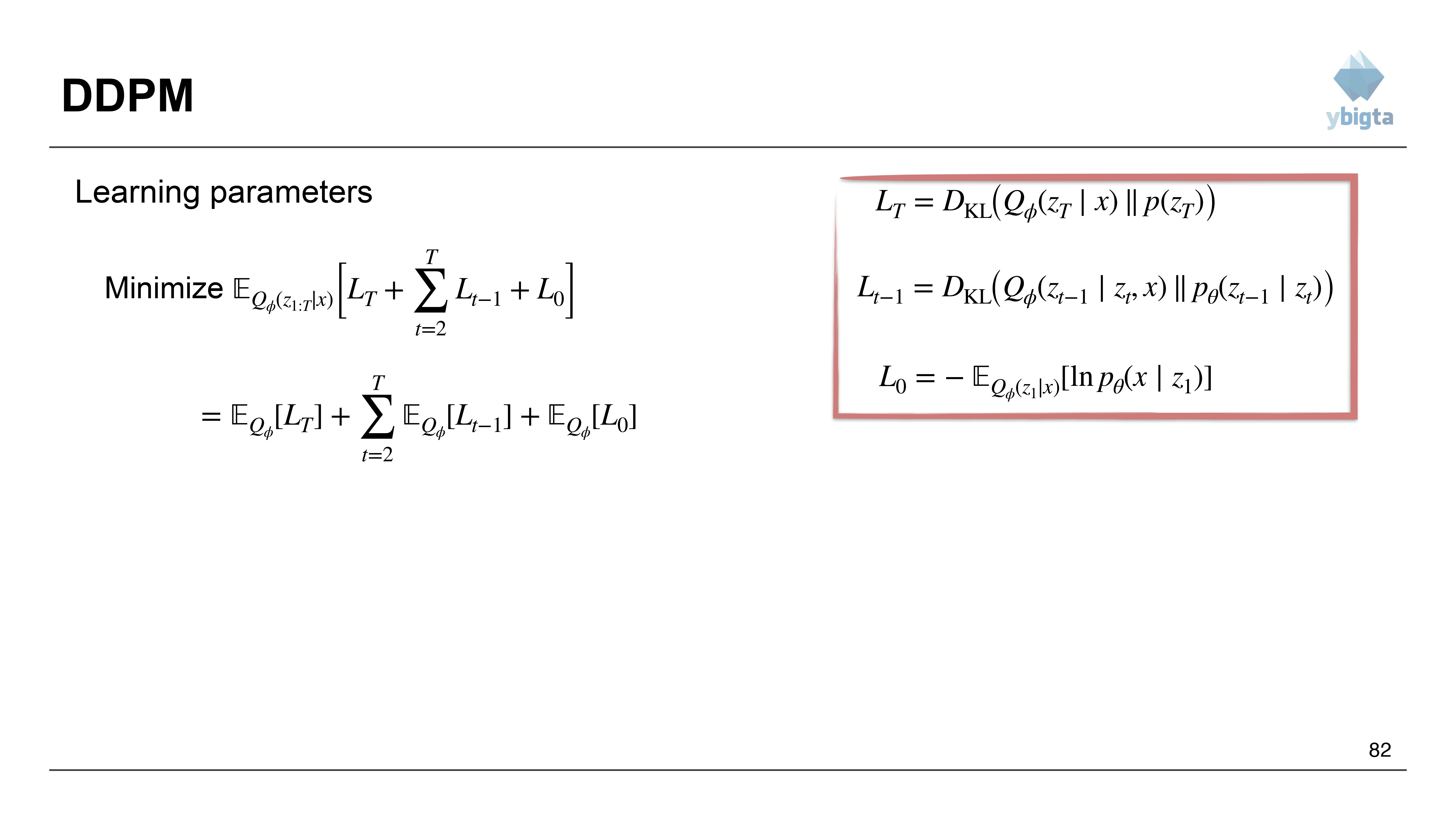
Slide 79: Loss Terms Definition
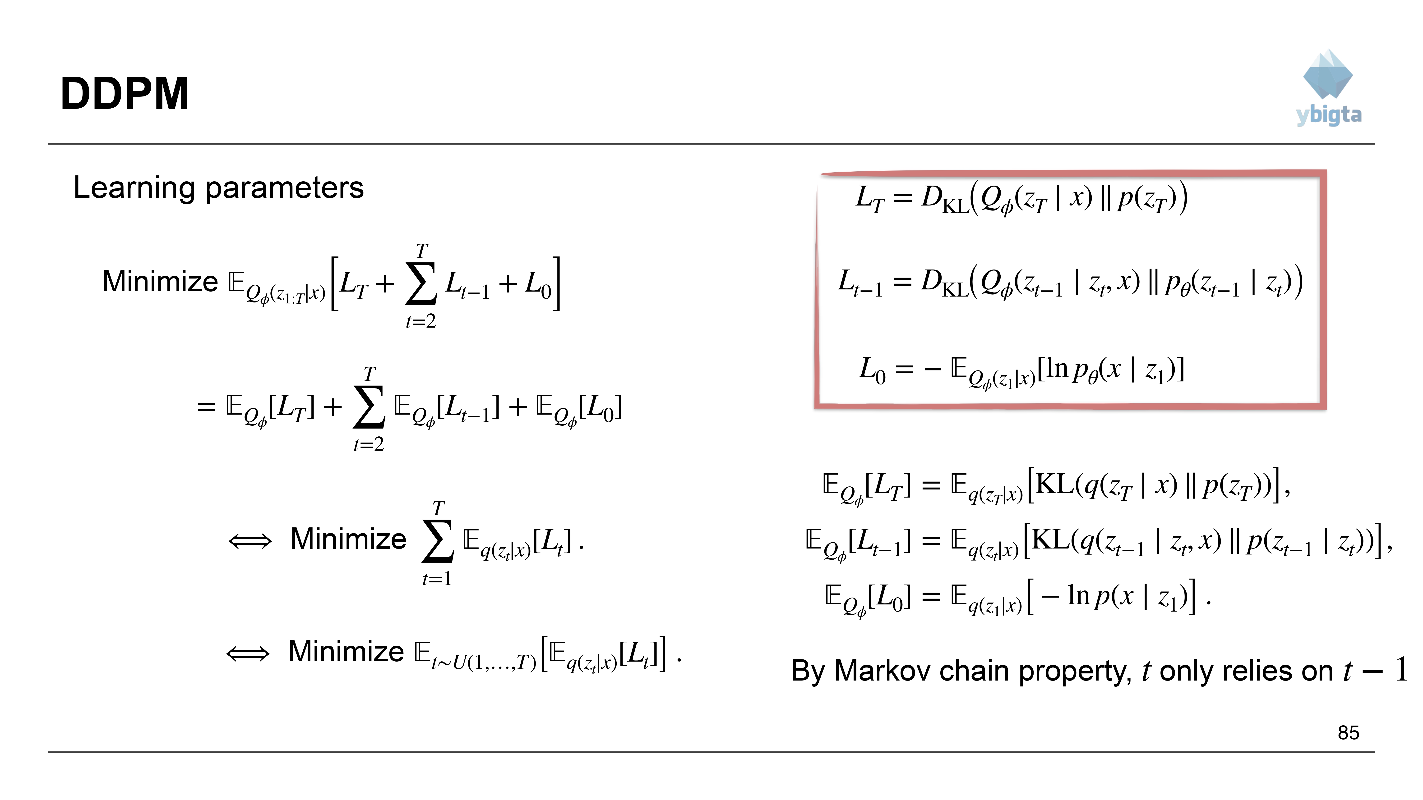
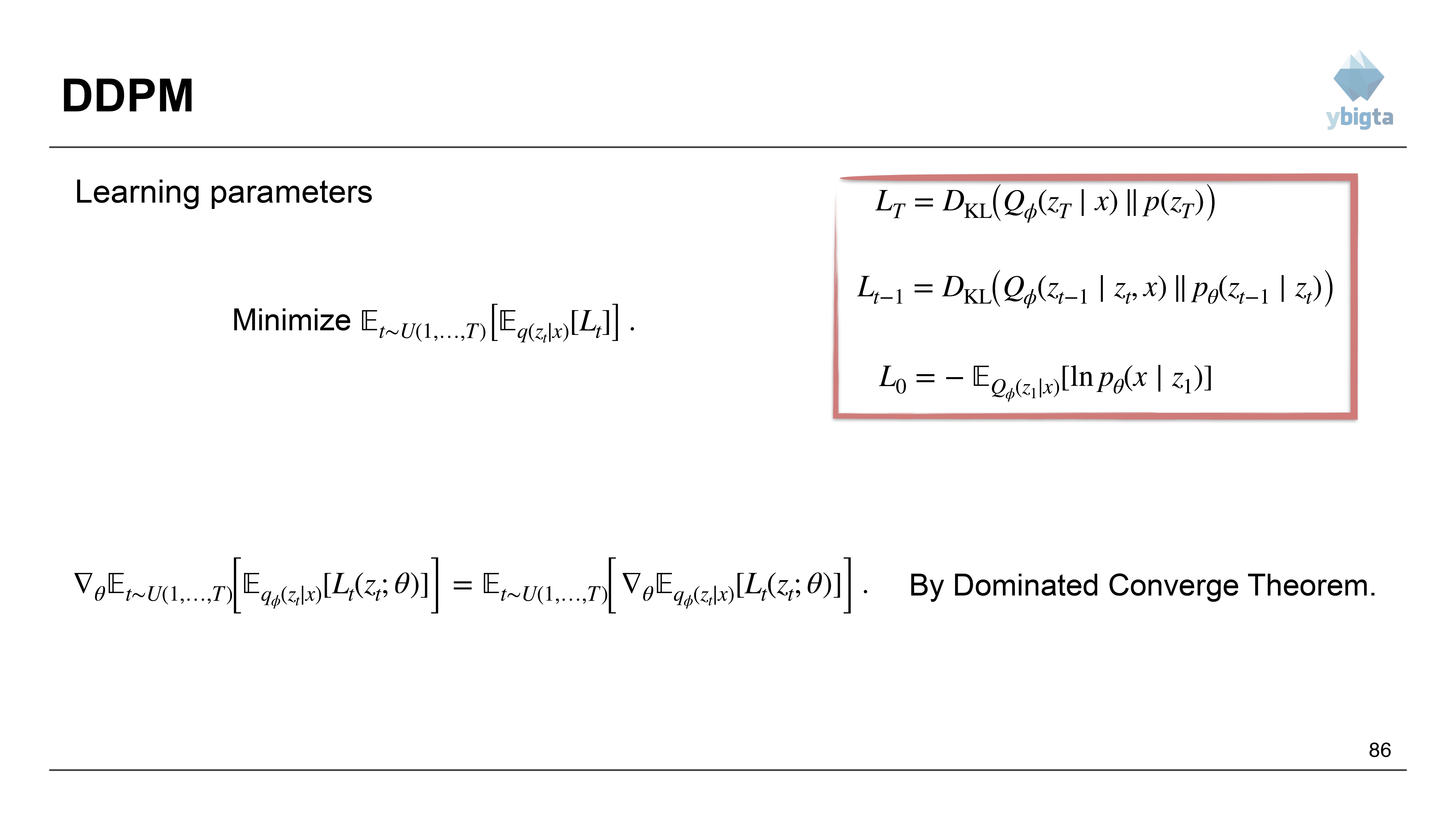
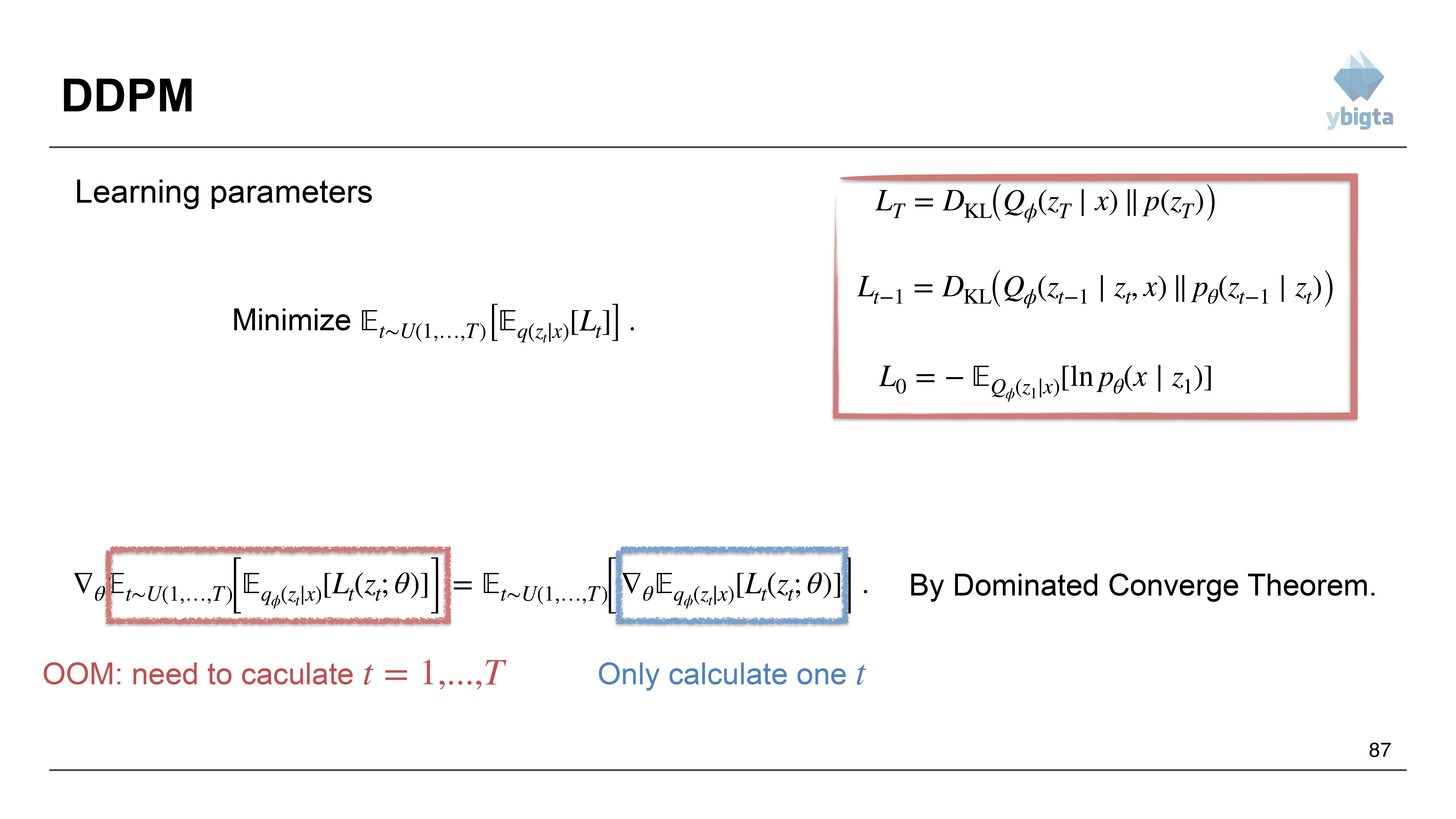
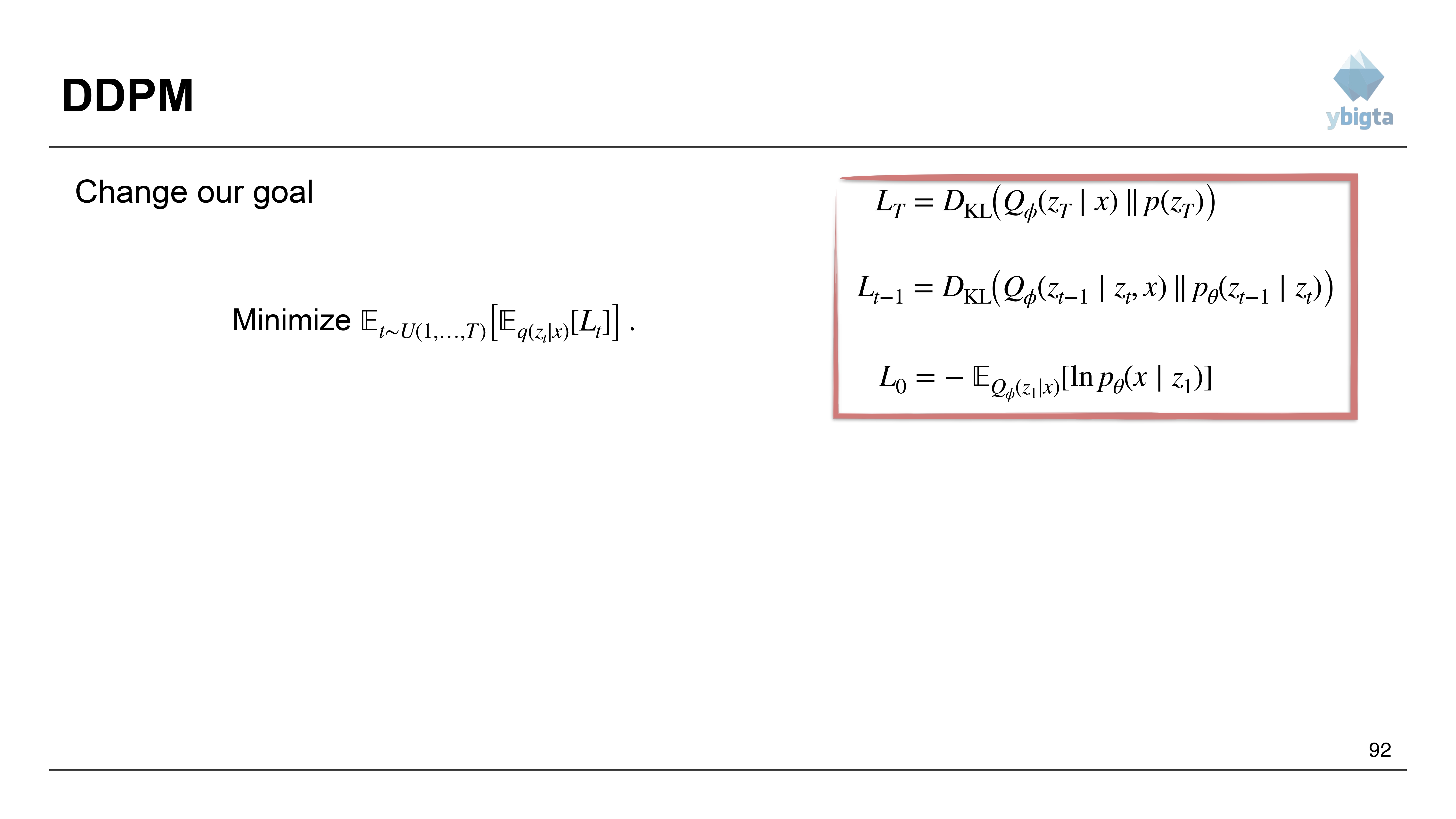
- $L_T = D_{KL}(Q_{\phi}(z_T|x) || p(z_T))$
- $L_{t-1} = D_{KL}(Q_{\phi}(z_{t-1}|z_t, x) || p_{\theta}(z_{t-1}|z_t))$
- $L_0 = -E_{Q}[ \ln p_{\theta}(x|z_1) ]$
- Total Loss: Minimize $\sum L$ terms.
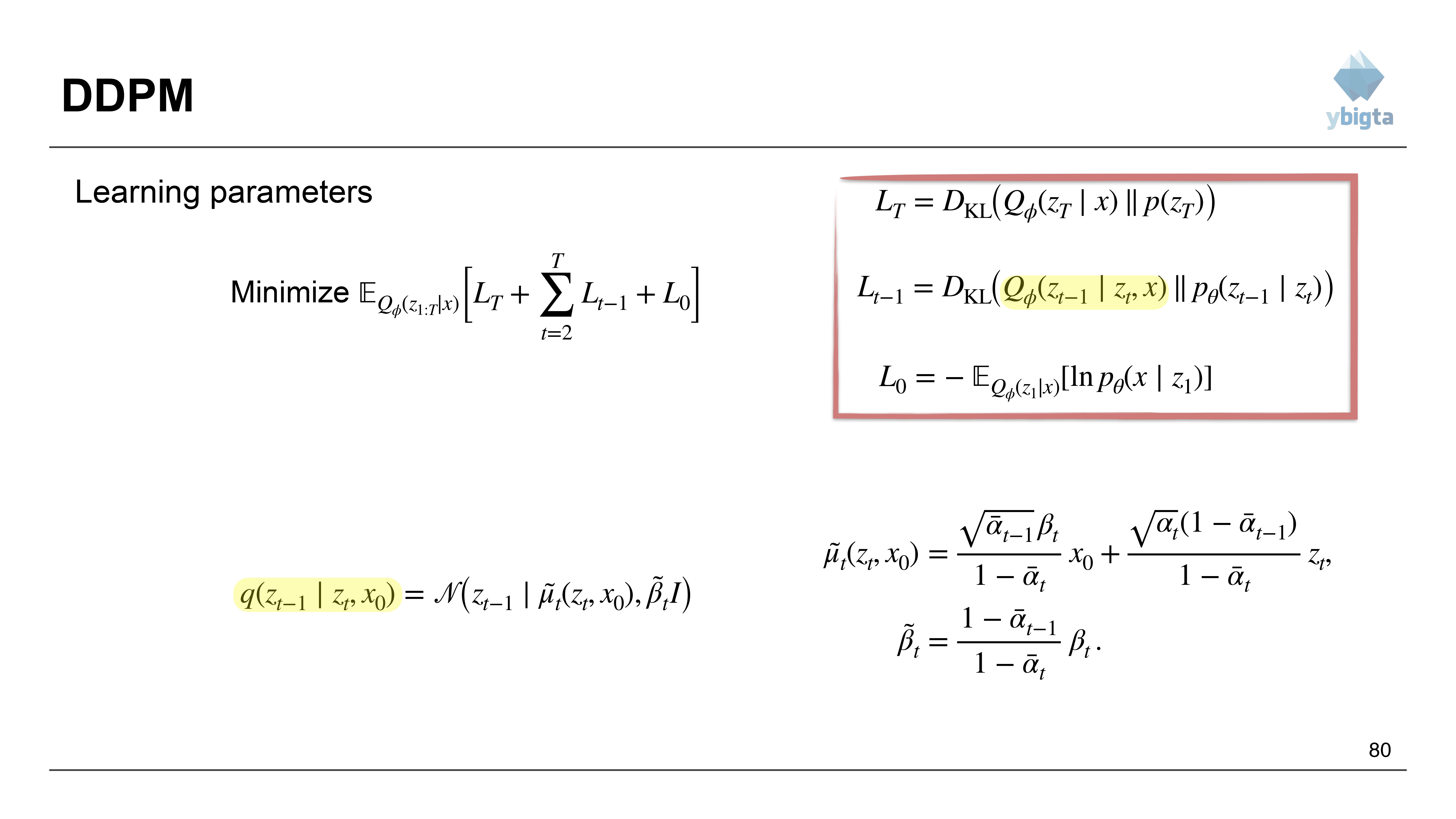
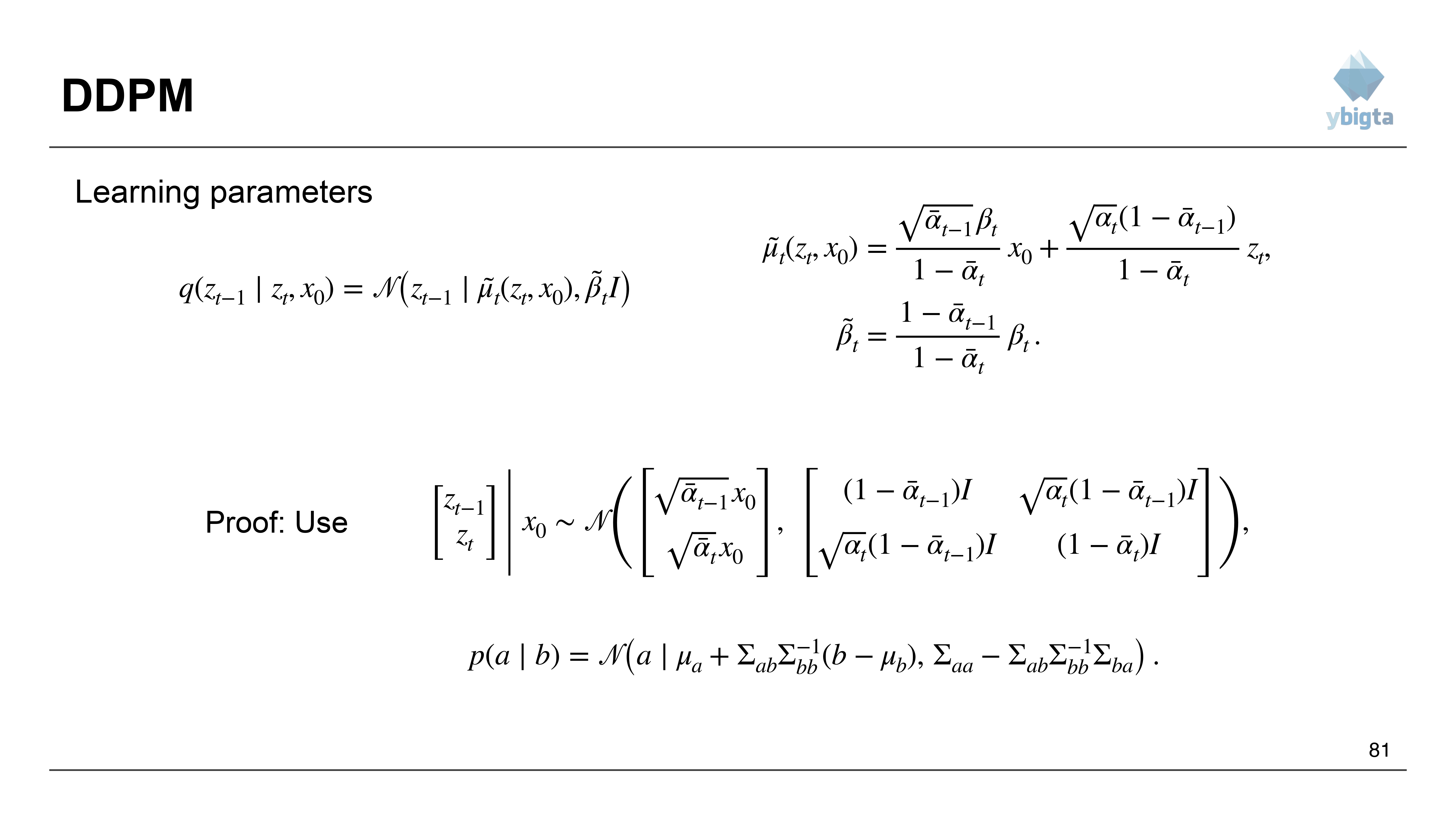
Slide 80: The Posterior $q(z_{t-1}|z_t, x_0)$
- This term $Q_{\phi}(z_{t-1}|z_t, x)$ is tractable!
- It is a Gaussian distribution $\mathcal{N}(\tilde{\mu}_t, \tilde{\beta}_t I)$.
- Mean $\tilde{\mu}_t$: A weighted combination of $x_0$ and $z_t$.
- Variance $\tilde{\beta}_t$: Function of $\beta$ and $\bar{\alpha}$.
Slide 81: Posterior Derivation
- Proof involves Gaussian conditioning formulas.
- Combining the forward equations allows us to solve for the distribution of $z_{t-1}$ given $z_t$ and $x_0$.
Slide 82: Loss Summation
- We sum the expectations of the loss terms.
Slide 83: Expectation Simplification
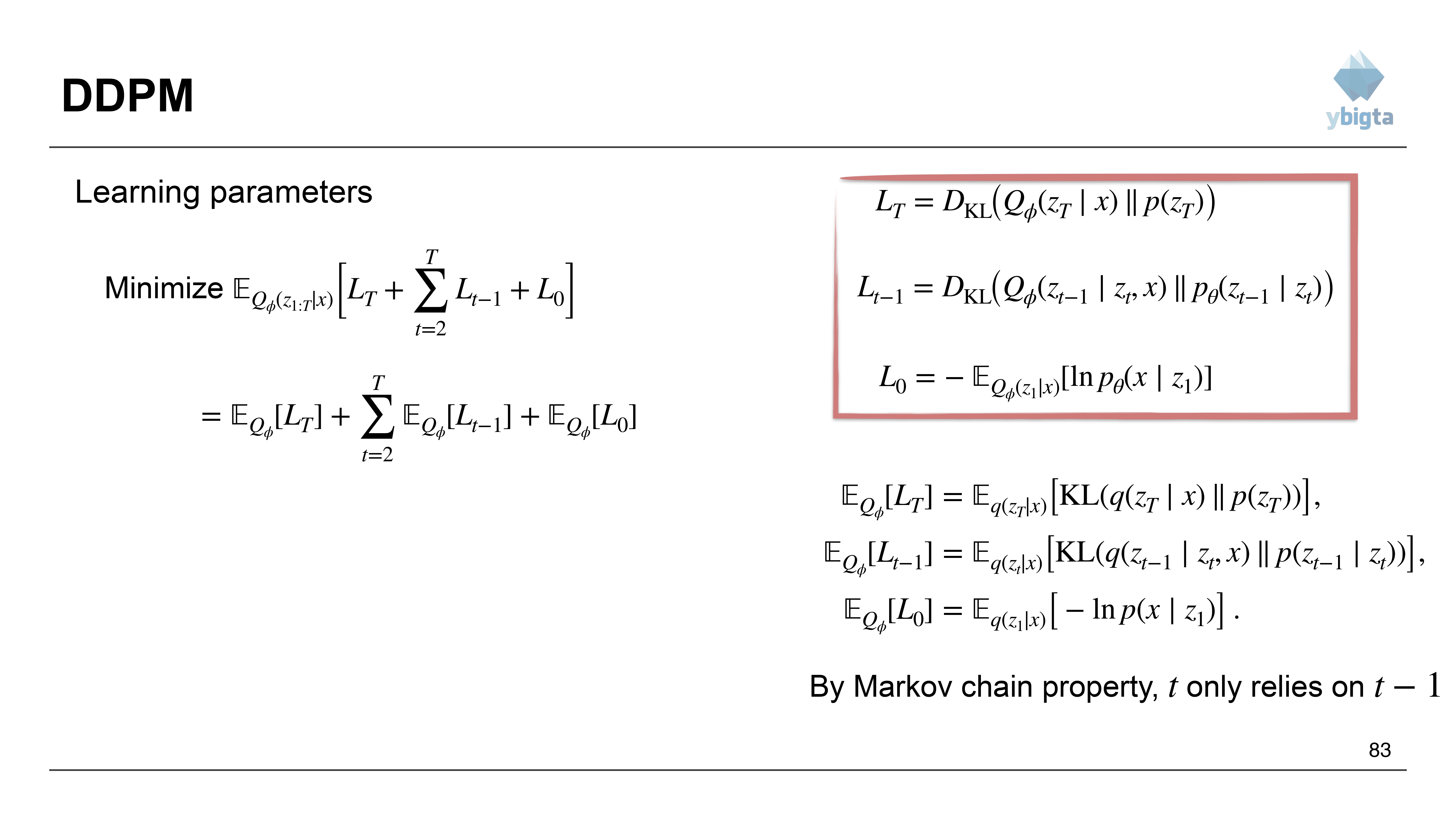
- $L_T$ relies on $z_T$.
- $L_{t-1}$ relies on $z_t, z_{t-1}$.
- By Markov chain property, we calculate expectations appropriately.
Slide 84: Minimization Objective
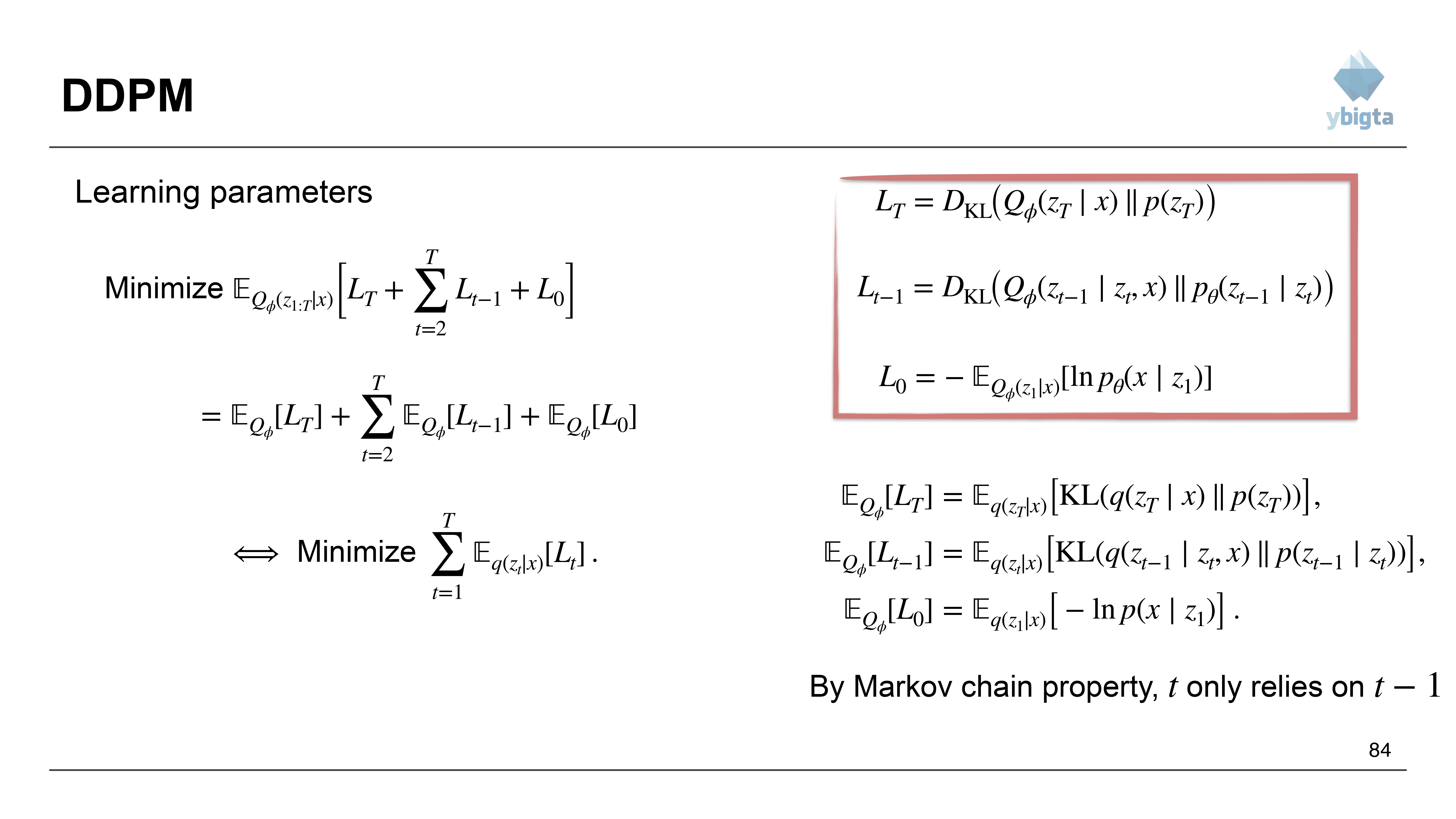
- Minimize $\sum_{t=1}^T \mathbb{E}_{q}[L_t]$.
Slide 85: Randomized Time Sampling
- Instead of summing all $T$ terms every step, we can sample $t \sim Uniform(1, \dots, T)$.
- Minimize $E_{t} [E_{q}[L_t]]$.
Slide 86: Gradient Descent
- We can take the gradient of this expected loss.
Slide 87: Efficient Training
- OOM: Calculating all $T$ steps is memory intensive.
- Solution: Only calculate one random $t$ per optimization step.
Slide 88: Analyzing the Loss
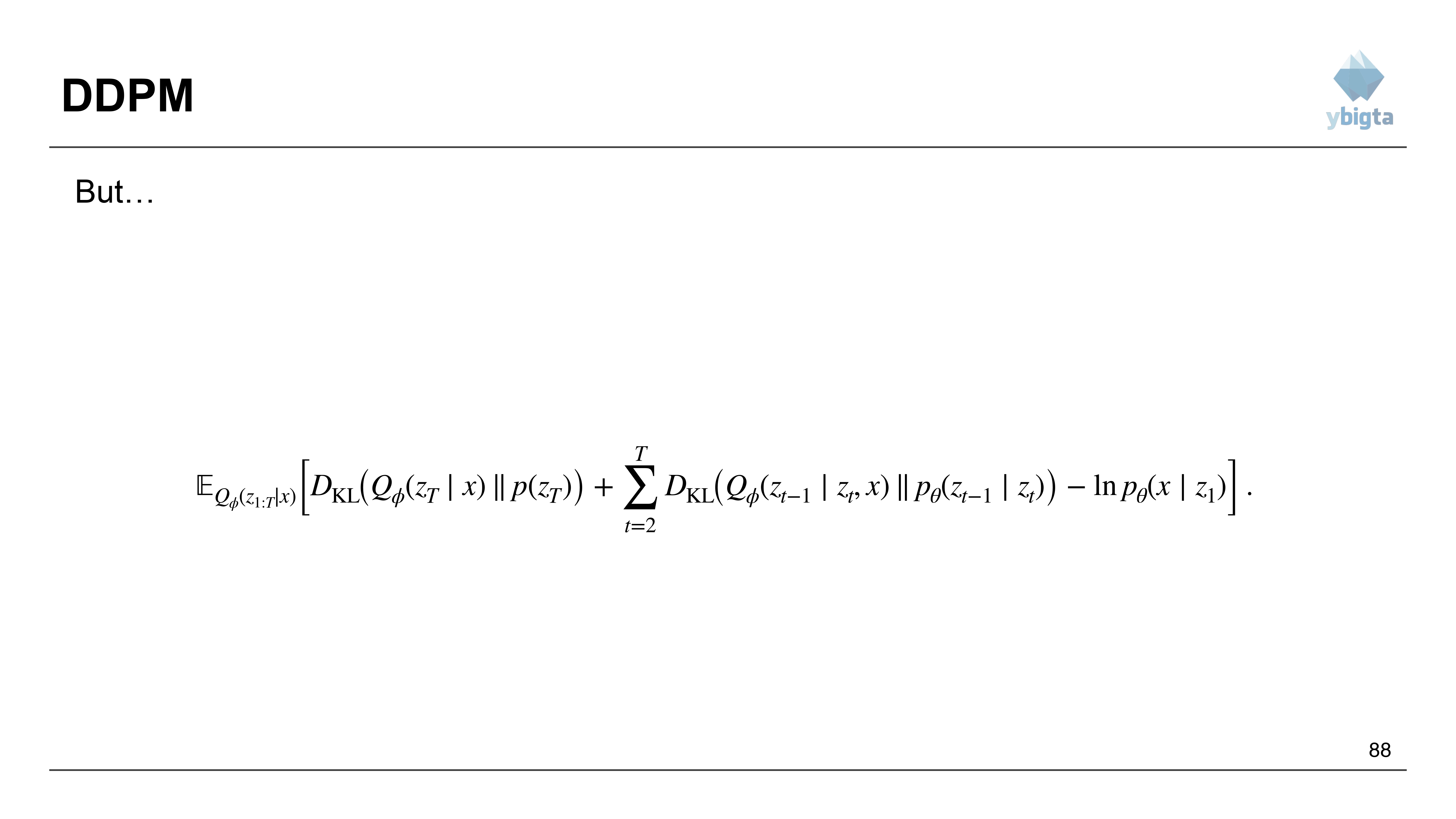
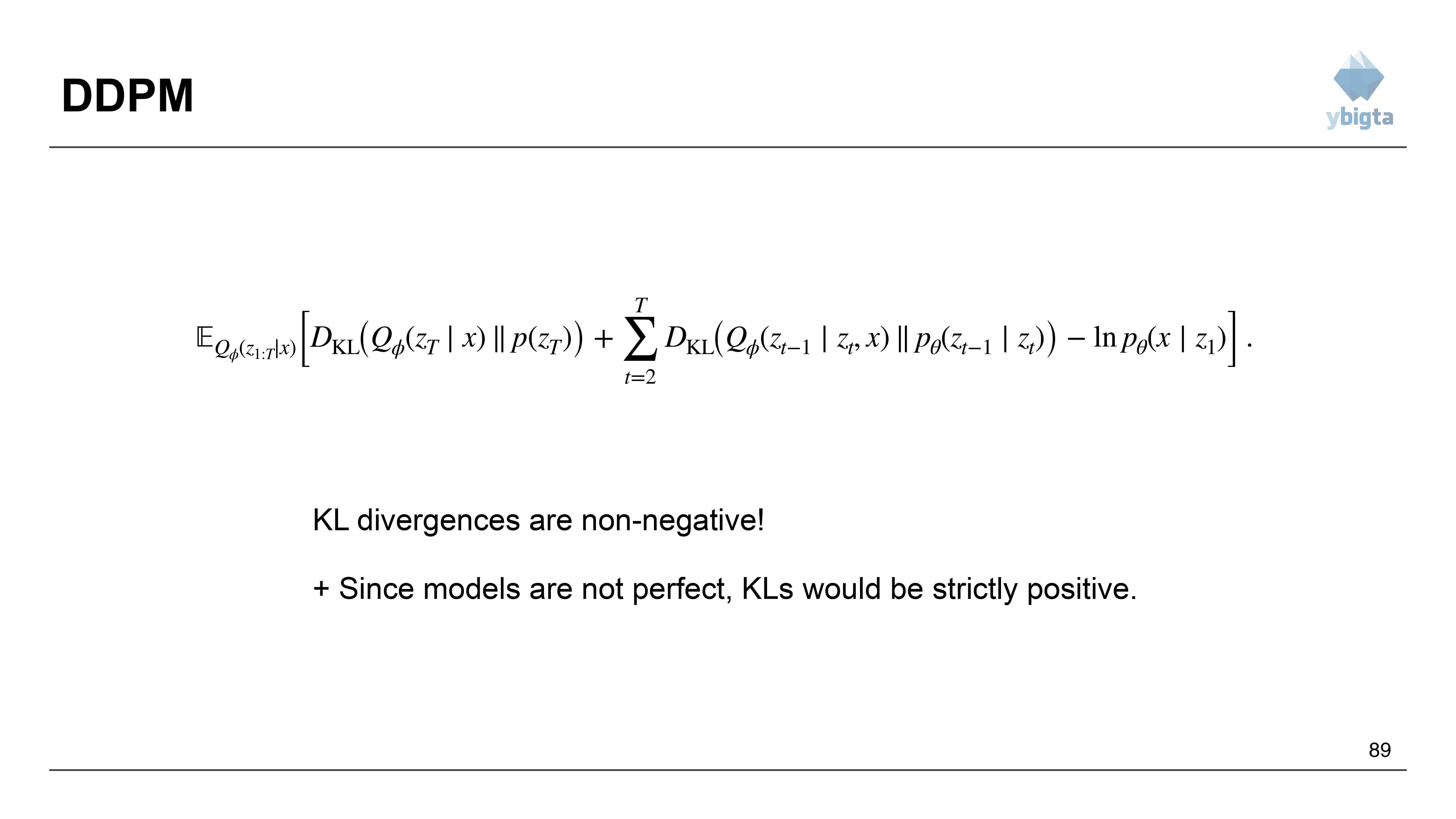
- Let’s look at the full ELBO equation again.
Slide 89: Positivity of KL
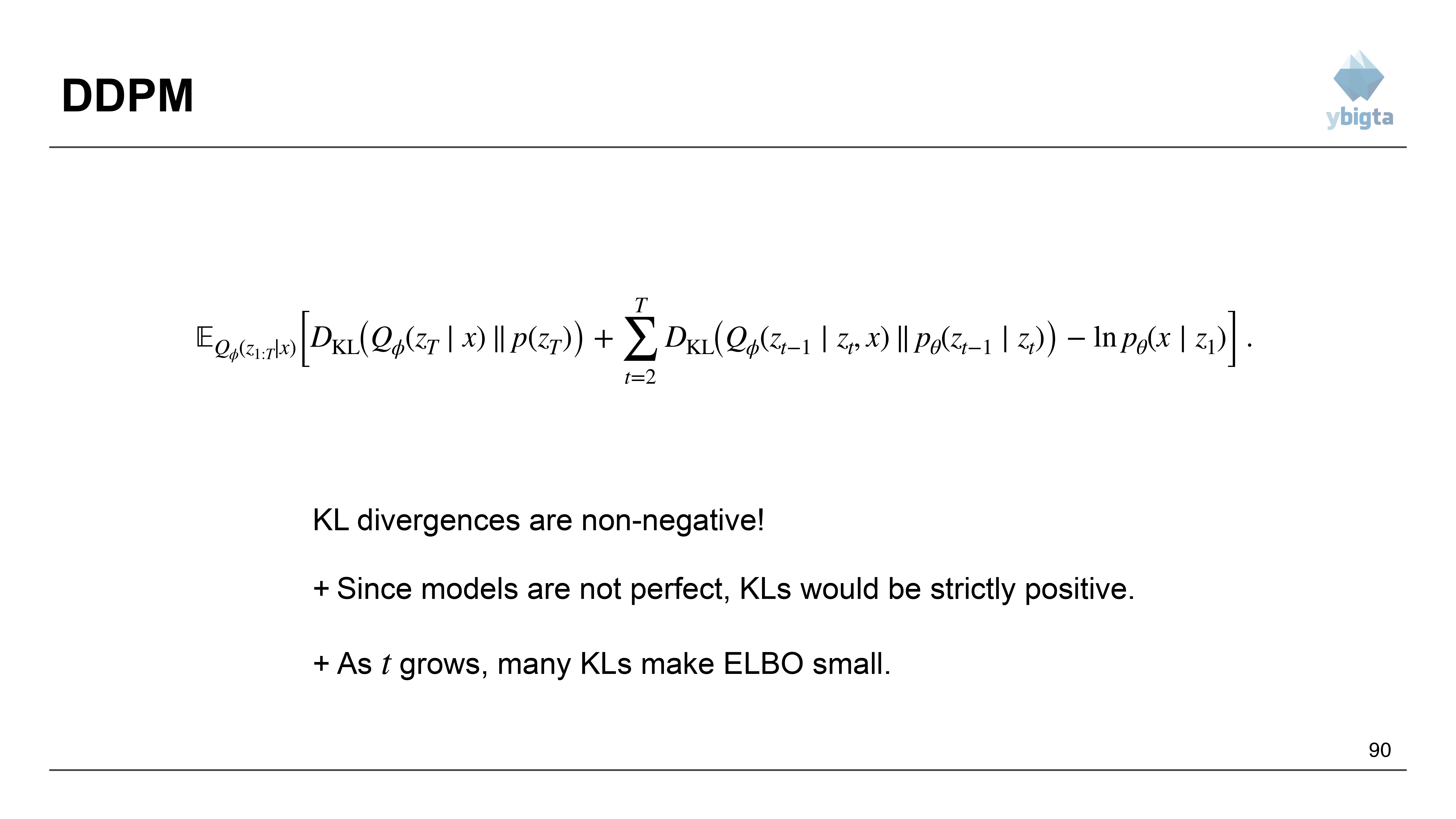
- KL divergences are non-negative.
- Since our models are not perfect approximations, these KL terms will be strictly positive.
Slide 90: Accumulation of Error
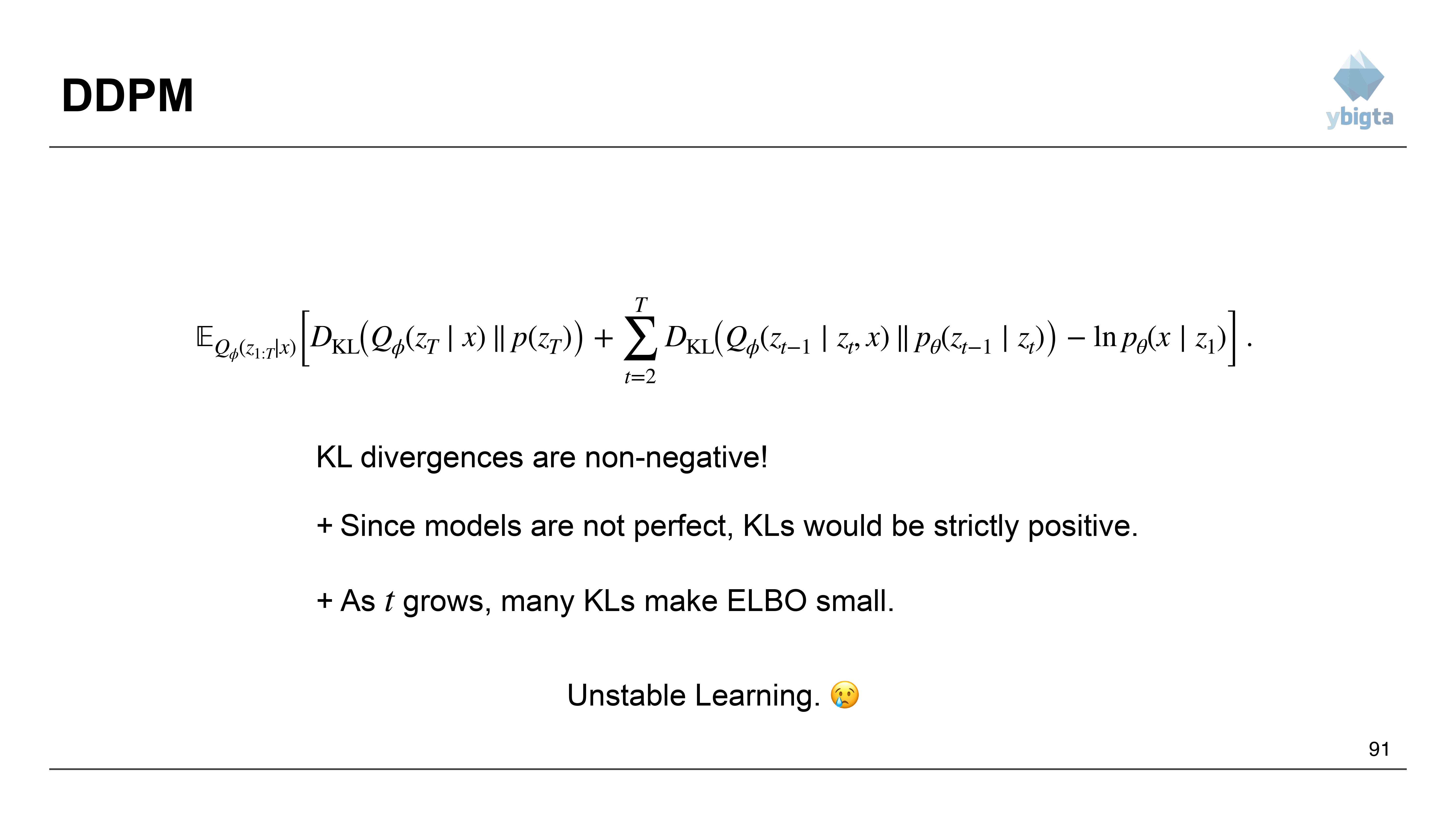
- As $T$ grows (many timesteps), there are many KL terms.
- This makes the ELBO value very small (large negative).
Slide 91: Unstable Learning
- Summing many KL terms can lead to variance issues and unstable learning.
Slide 92: Changing the Goal
- We focus on the specific term: $L_{t-1} = D_{KL}(Q(z_{t-1}|z_t, x) || p_{\theta}(z_{t-1}|z_t))$.
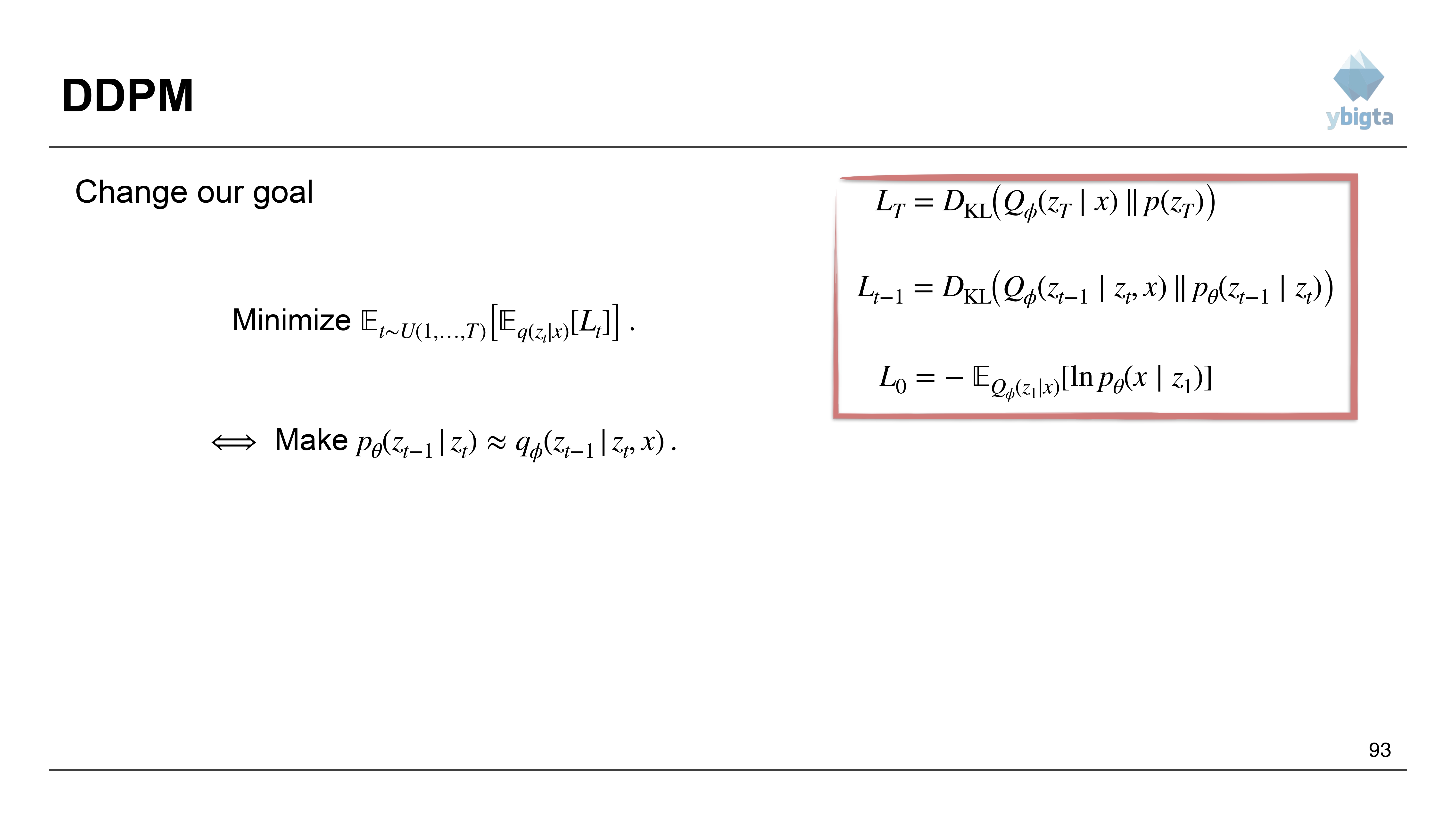
Slide 93: Matching Distributions
- Our goal is to make the learned reverse process $p_{\theta}(z_{t-1}|z_t)$ approximate the true posterior $q_{\phi}(z_{t-1}|z_t, x)$.
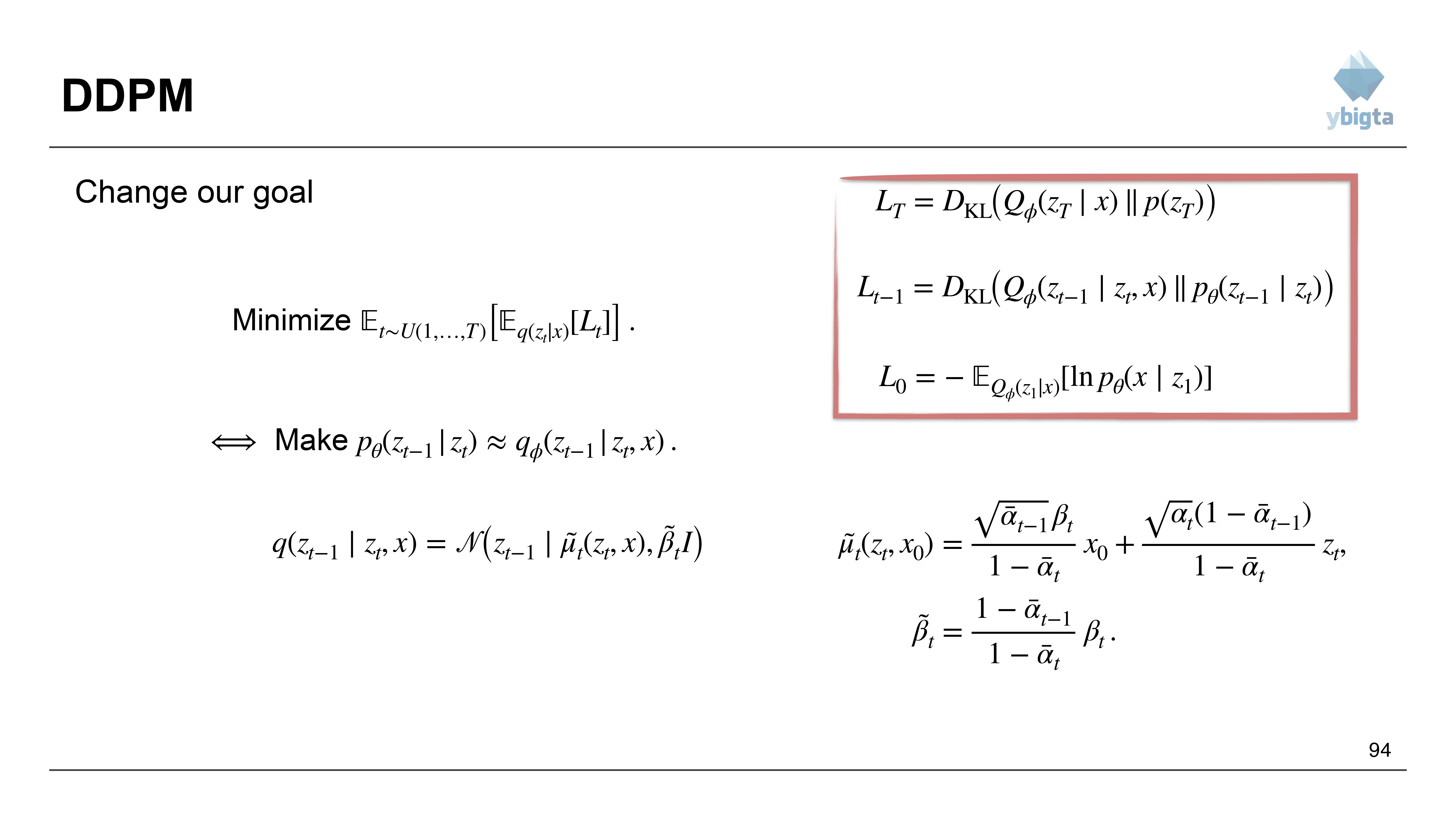
Slide 94: Gaussian Matching
- Both distributions are Gaussian.
- $q \sim \mathcal{N}(\tilde{\mu}_t, \tilde{\beta}_t I)$
- $p_{\theta} \sim \mathcal{N}(\mu_{\theta}, \sigma_t^2 I)$ (Usually $\sigma_t^2$ is fixed to $\beta_t$ or $\tilde{\beta}_t$).
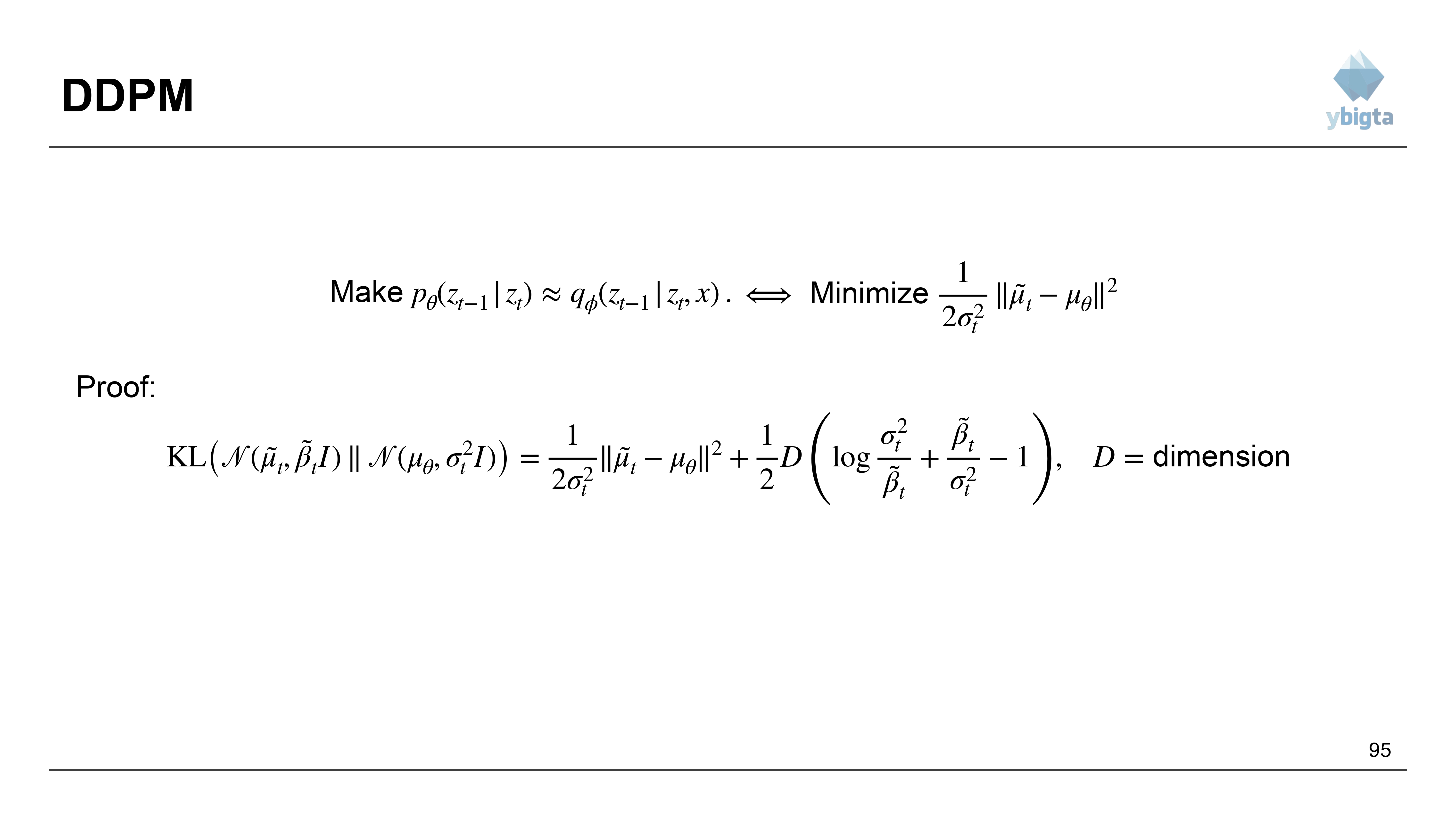
Slide 95: KL between Gaussians
- The KL divergence between two Gaussians with diagonal covariance is proportional to the MSE of their means.
- Minimize:
$$
\frac{1}{2\sigma_t^2} \left\lVert \tilde{\mu}_t - \mu_{\theta} \right\rVert^2
$$
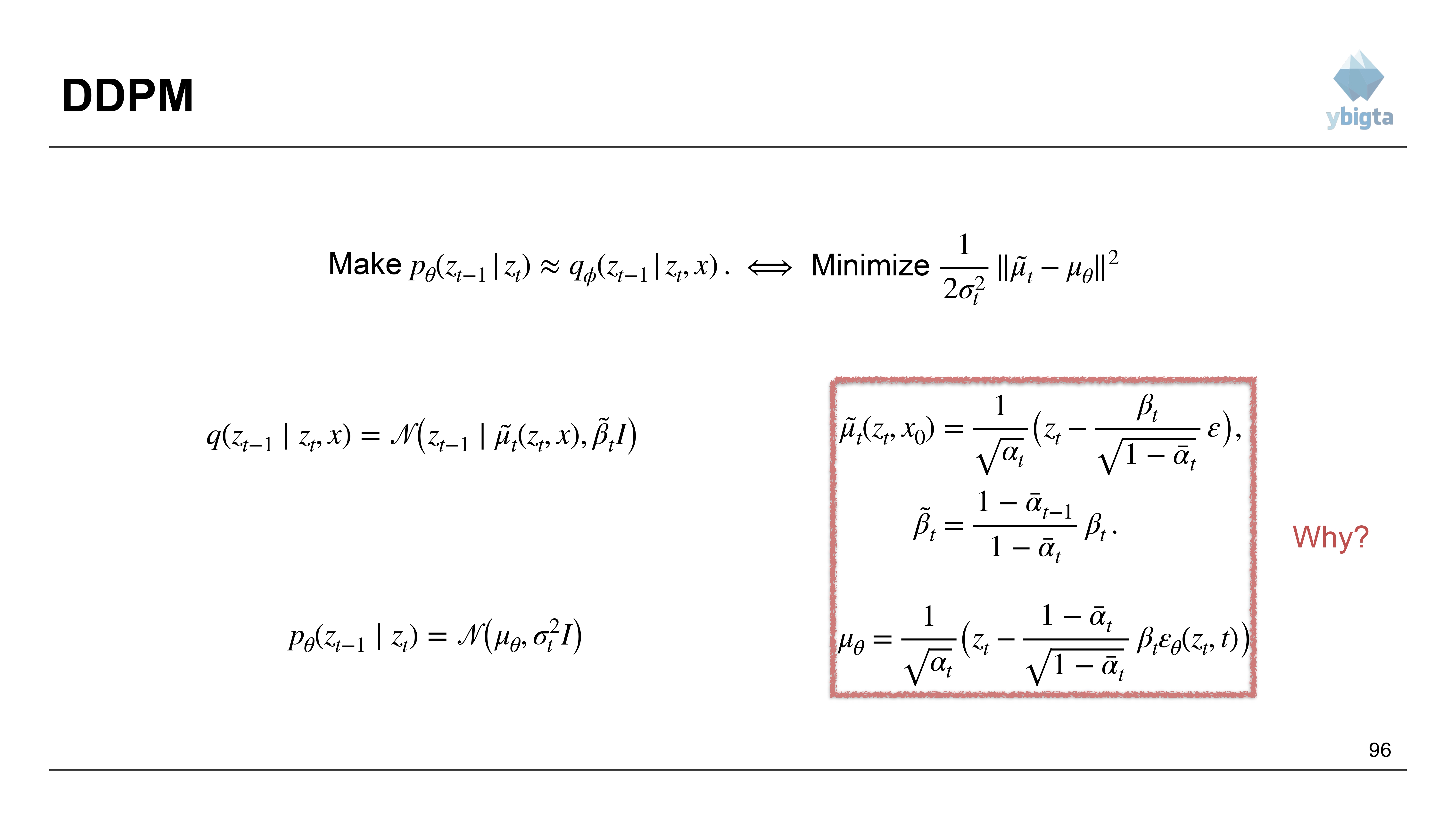
Slide 96: Parametrization of $\mu_{\theta}$
- We know $\tilde{\mu}_t(z_t, x)$ can be written in terms of $z_t$ and the noise $\epsilon$ used to generate it.
- $\tilde{\mu}_t = \frac{1}{\sqrt{\alpha_t}} (z_t - \frac{\beta_t}{\sqrt{1-\bar{\alpha}_t}}\epsilon)$
- So, we should parameterize $\mu_{\theta}$ to predict $\epsilon$!
$$
\mu_{\theta} = \frac{1}{\sqrt{\alpha_t}} \left(z_t - \frac{\beta_t}{\sqrt{1-\bar{\alpha}_t}}\epsilon_{\theta}(z_t, t)\right)
$$
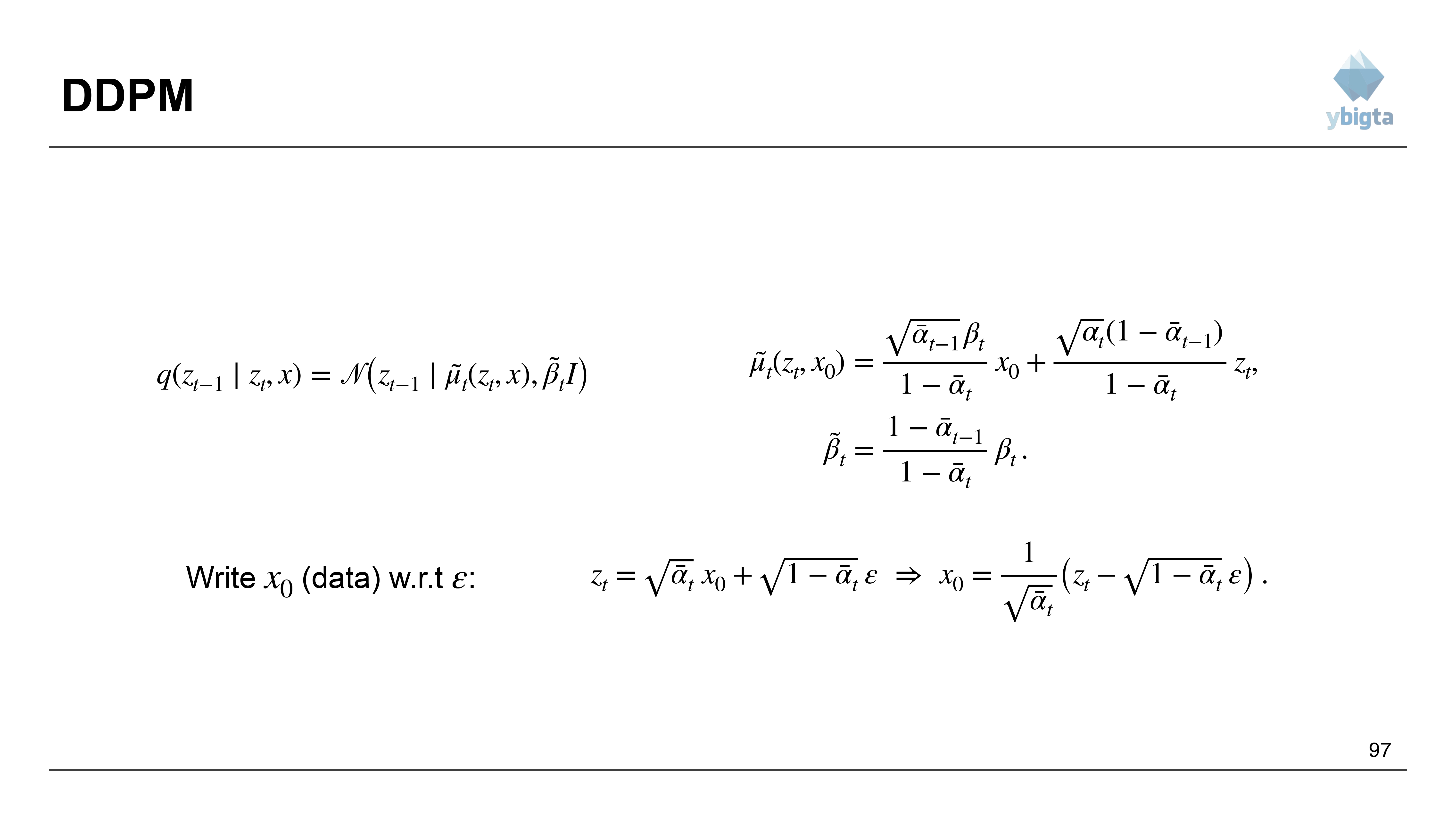
Slide 97: Derivation Step 1
- Recall the definition of $\tilde{\mu}_t$ (weighted average of $x_0$ and $z_t$).
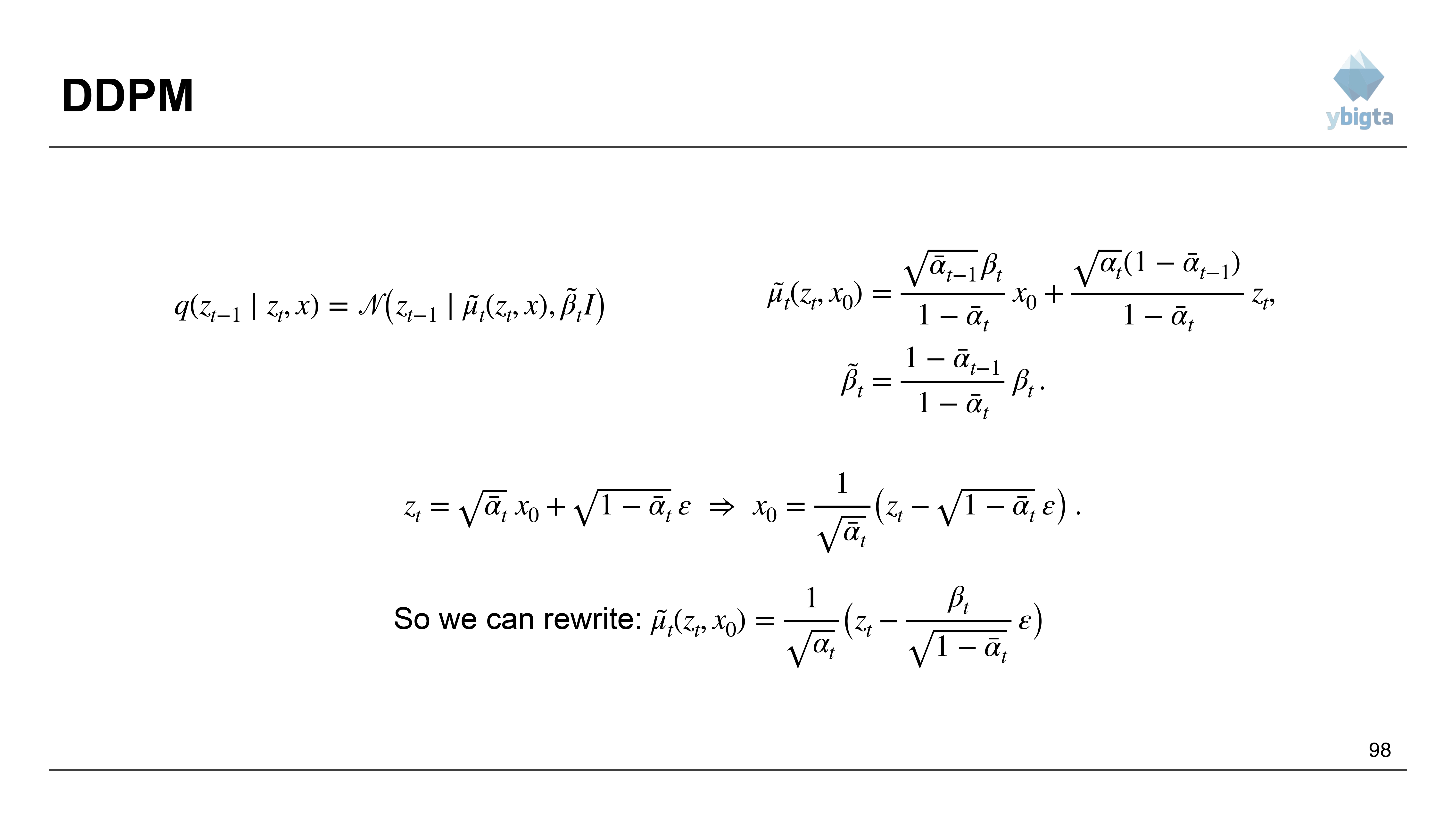
Slide 98: Derivation Step 2
- Substitute $x_0$ with its expression derived from $z_t$ and $\epsilon$.
- $x_0 = \frac{1}{\sqrt{\bar{\alpha}_t}}(z_t - \sqrt{1-\bar{\alpha}_t}\epsilon)$
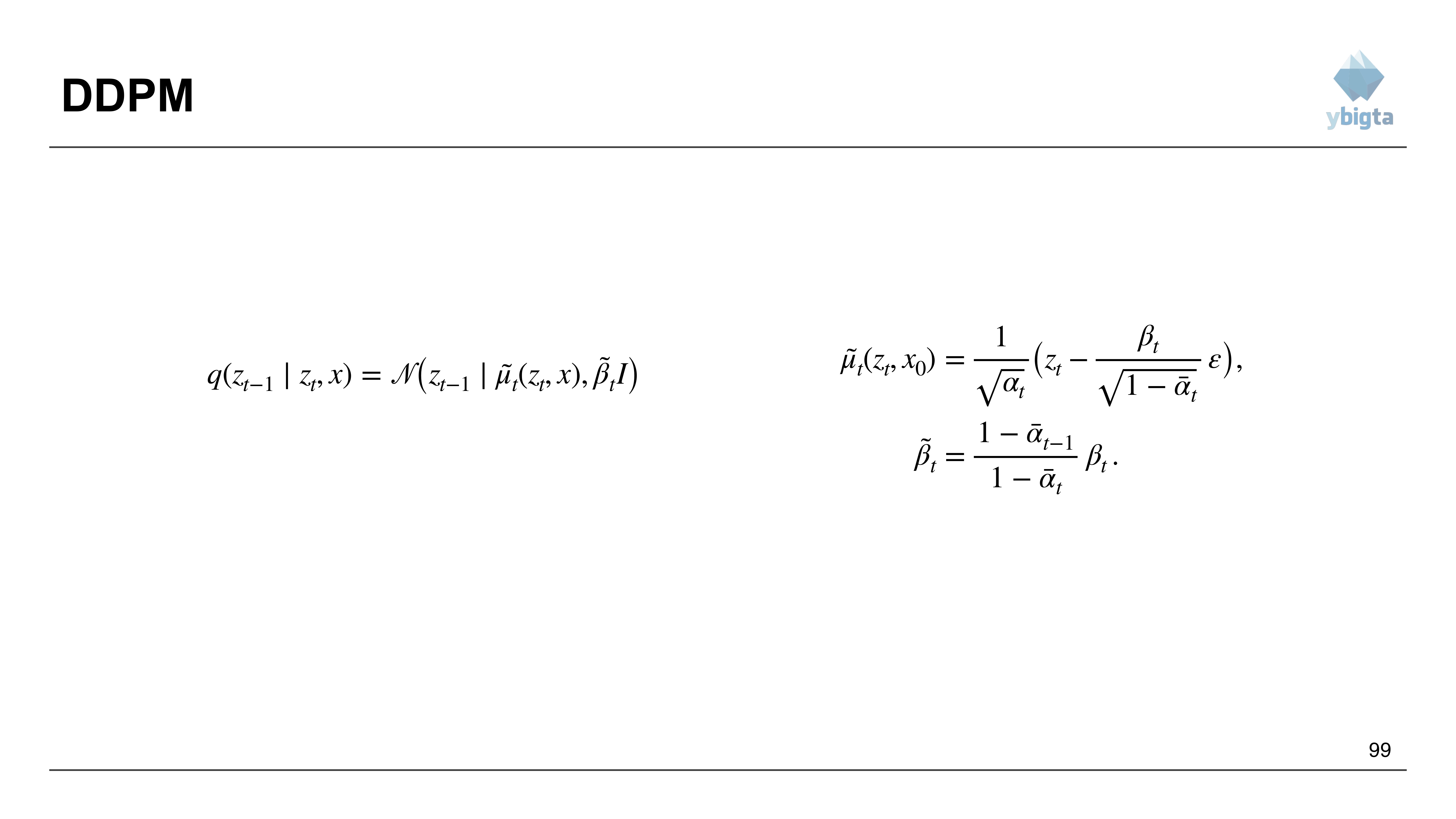
Slide 99: Derivation Step 3
- Simplify the algebra to get the expression for $\tilde{\mu}_t$ solely in terms of $z_t$ and $\epsilon$.
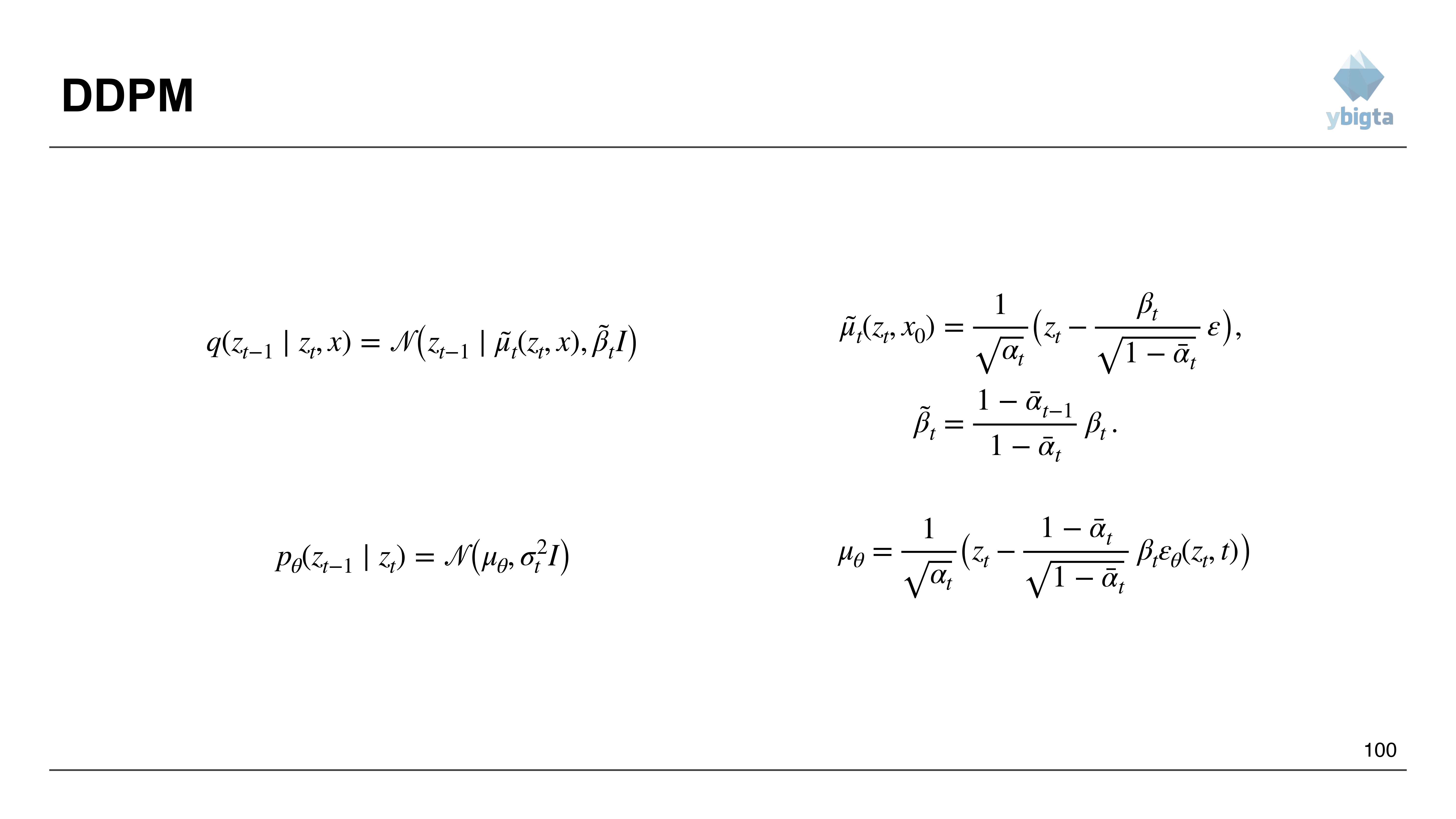
Slide 100: Matching Means
$$
\text{Since }\tilde{\mu}_t\text{ depends on }\epsilon\text{, our model }\mu_{\theta}\text{ should approximate it by using a neural network }\epsilon_{\theta}(z_t, t)\text{ to predict that noise.}
$$
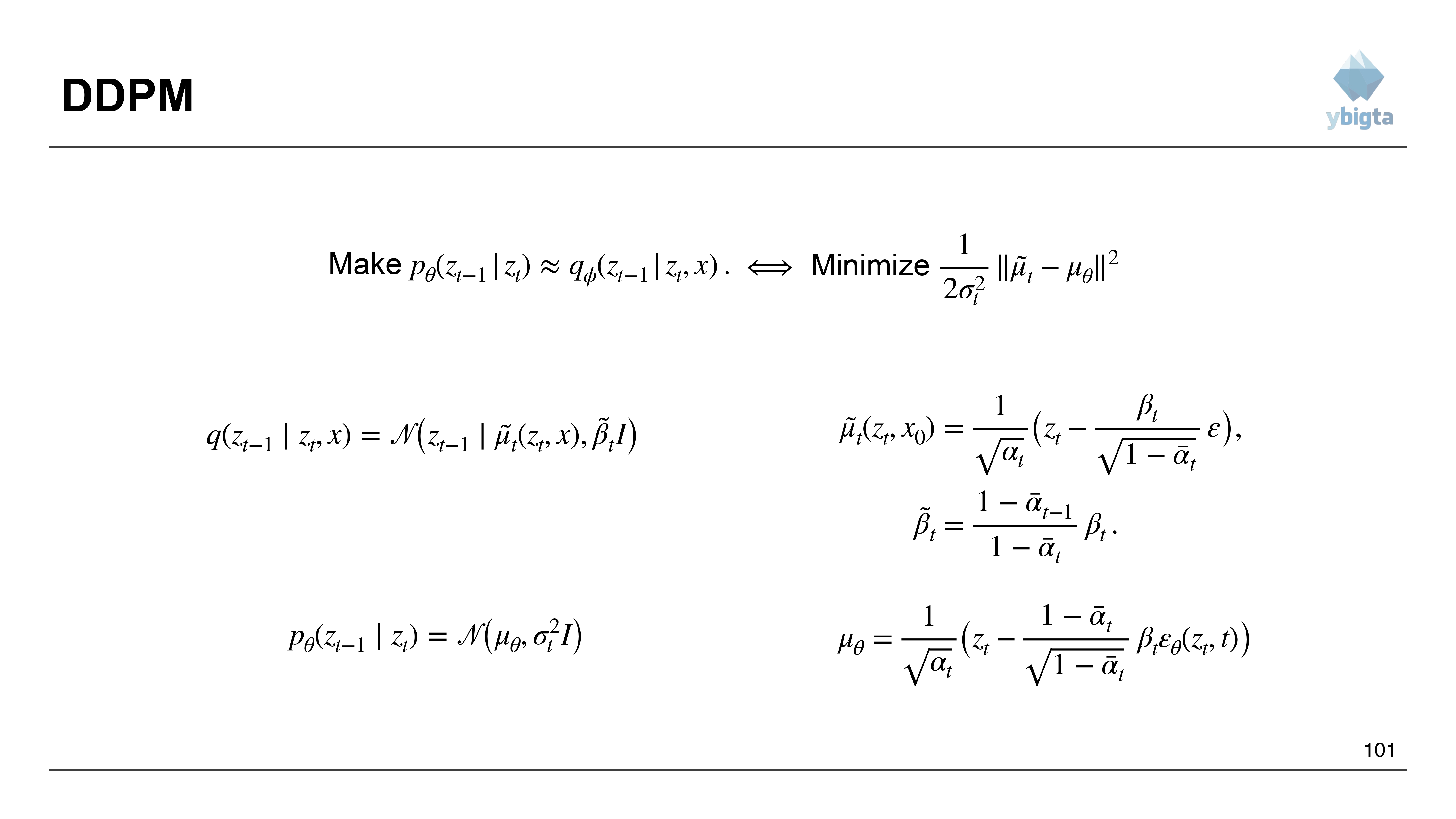
Slide 101: Comparison
$$
\text{Comparison of the target mean }\tilde{\mu}_t\text{ and the model mean }\mu_{\theta}\text{.}
$$
- They are identical in form, except one uses true noise $\epsilon$ and the other uses predicted noise $\epsilon_{\theta}$.
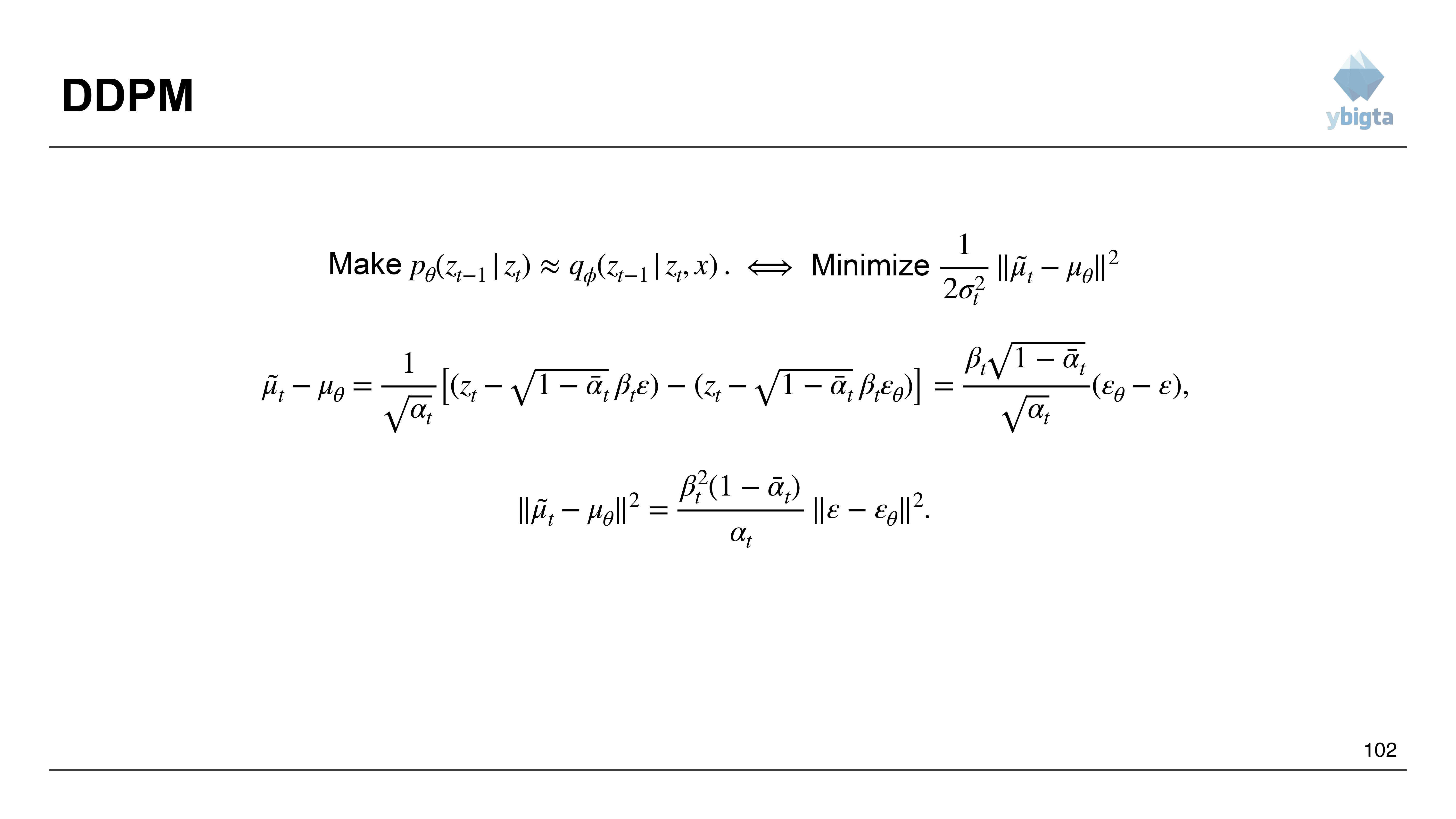
Slide 102: Difference of Means
$$
\text{Calculating }\tilde{\mu}_t - \mu_{\theta}\text{.}
$$
- Everything cancels out except the noise terms.
- Difference $\propto (\epsilon - \epsilon_{\theta})$.
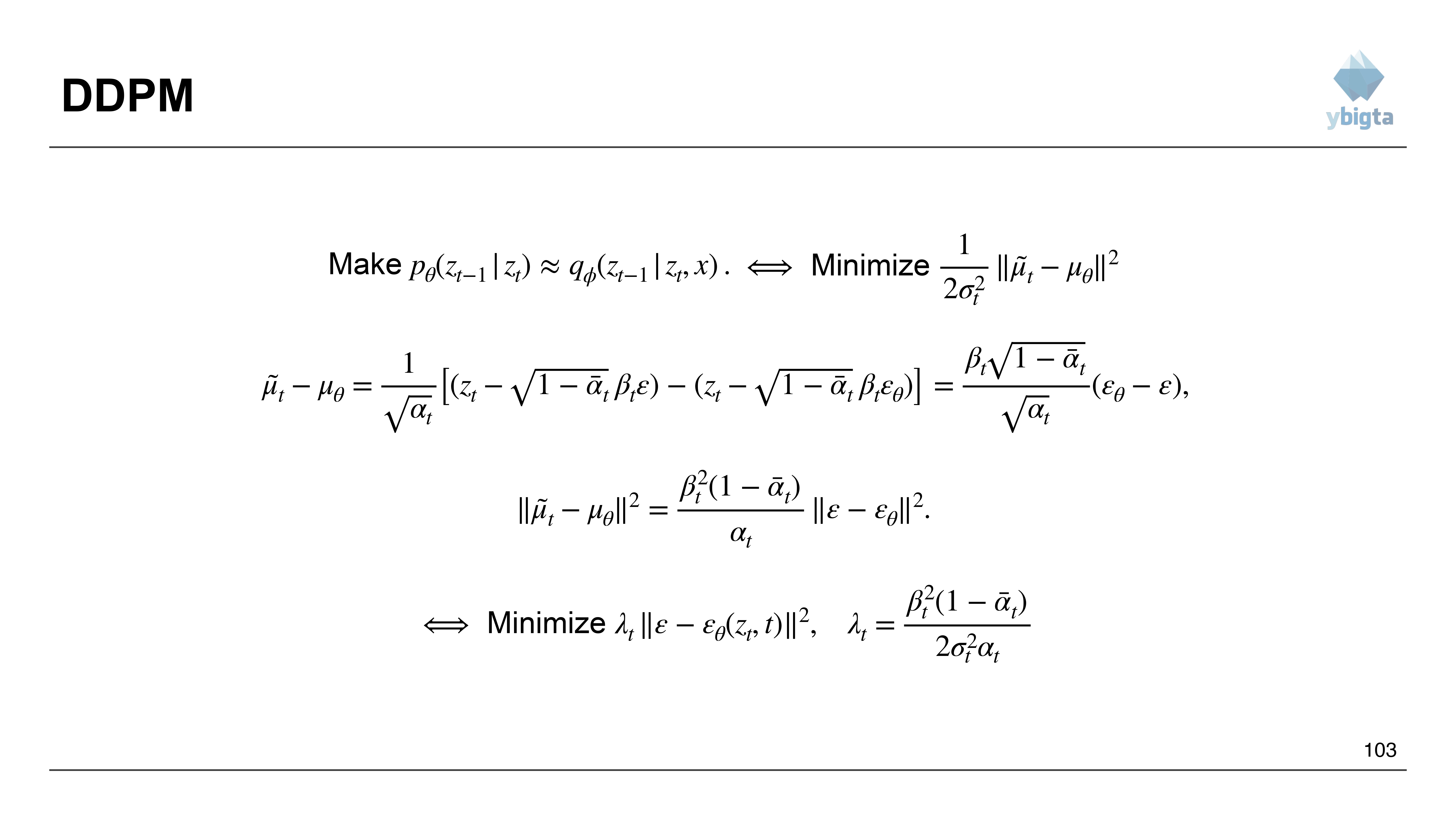
Slide 103: Simplified Loss Function
- The loss becomes weighted MSE between true noise and predicted noise.
$$
L_{simple} = \mathbb{E}_{t, x_0, \epsilon} \left[ \left\lVert \epsilon - \epsilon_{\theta}\big(\sqrt{\bar{\alpha}_t}x_0 + \sqrt{1-\bar{\alpha}_t}\,\epsilon, t\big) \right\rVert^2 \right]
$$
- $\lambda_t$ is a weighting term derived from the variances.
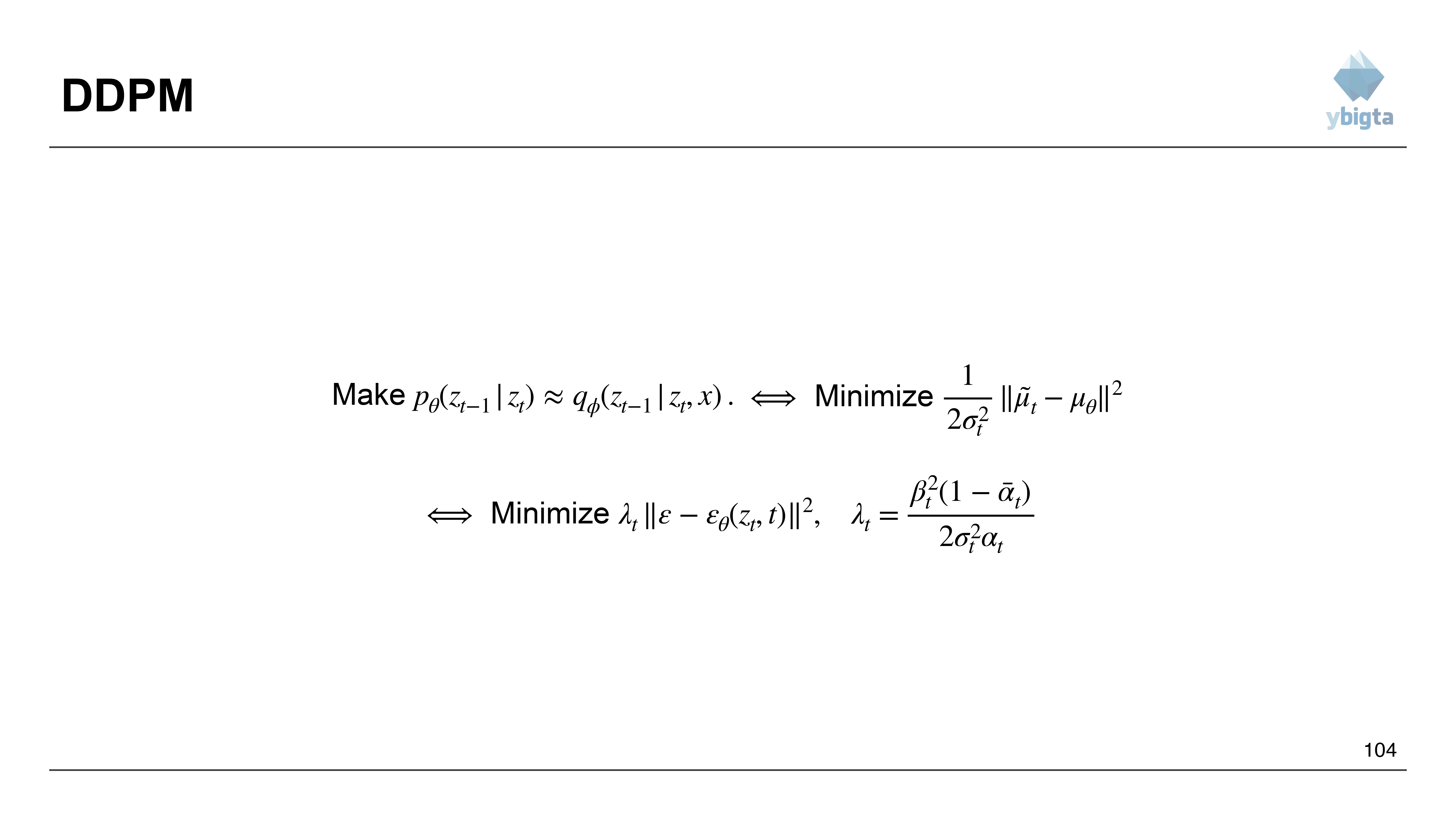
Slide 104: Final Simplification
- Ho et al. (DDPM) found that ignoring the weighting term $\lambda_t$ (setting it to 1) works better in practice.
- It puts more weight on difficult aspects of the denoising task.
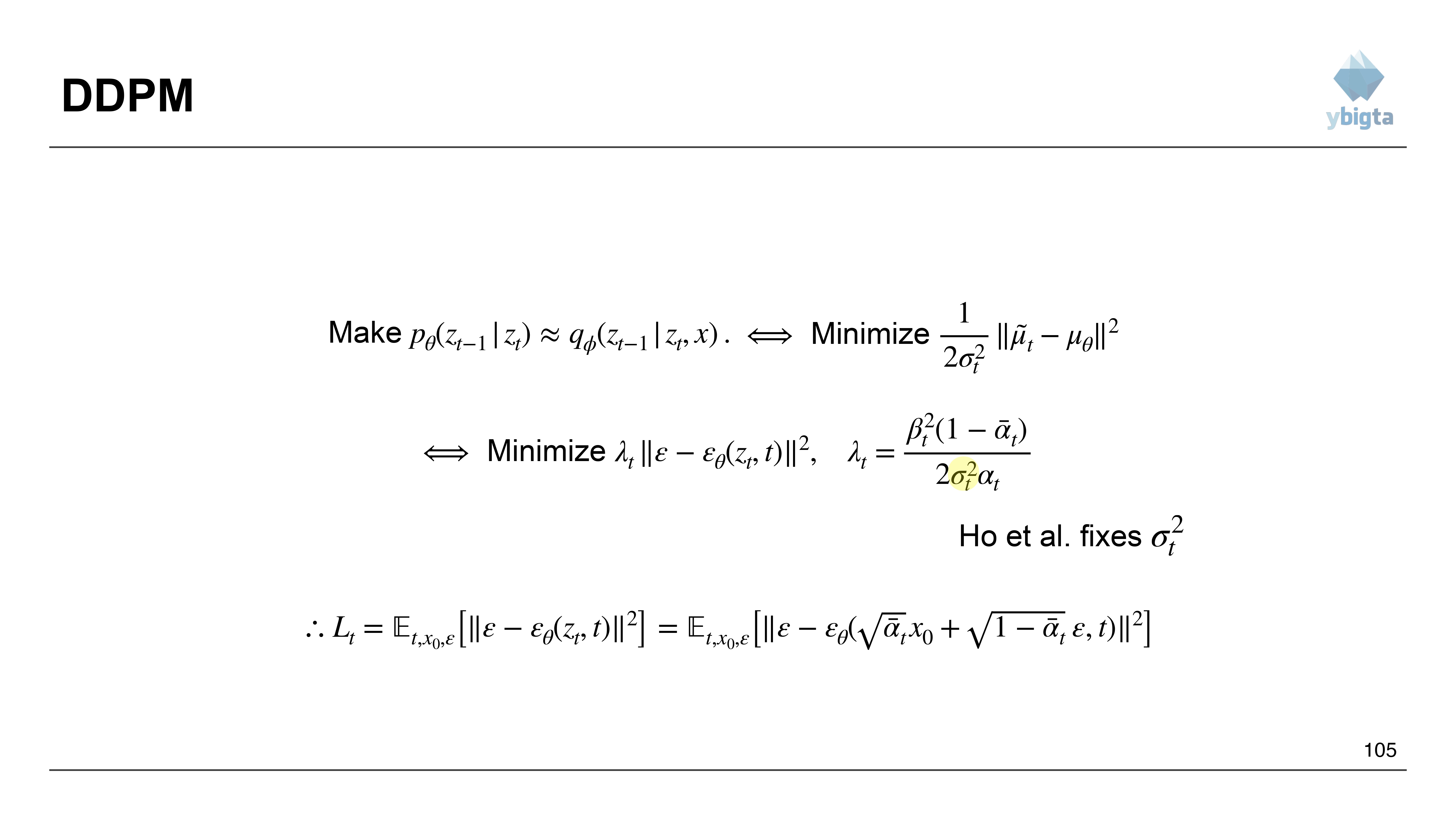
Slide 105: The “Simple” Loss
$$
L_{simple} = \mathbb{E}_{t, x_0, \epsilon} \left[ \left\lVert \epsilon - \epsilon_{\theta}\big(\sqrt{\bar{\alpha}_t}x_0 + \sqrt{1-\bar{\alpha}_t}\epsilon, t\big) \right\rVert^2 \right]
$$
- We simply train a network to predict the noise added to the image.
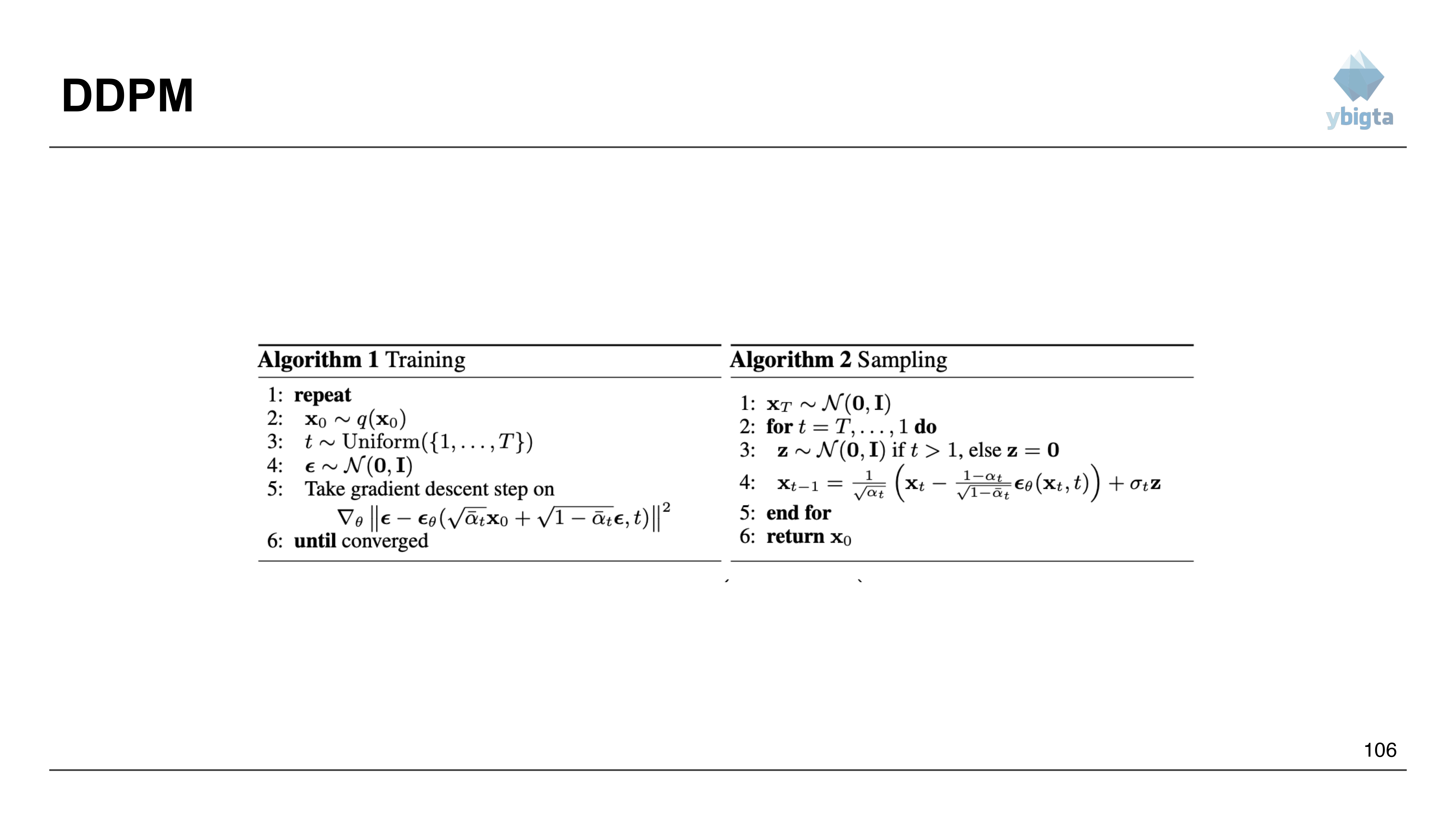
Slide 106: Algorithms
- Algorithm 1 (Training):
- Sample $x_0$.
- Sample $t$.
- Sample noise $\epsilon$.
- Gradient descent on $|| \epsilon - \epsilon_{\theta}(\text{noisy input}, t) ||^2$.
- Algorithm 2 (Sampling):
- Start from $x_T \sim \mathcal{N}(0, I)$.
- Iteratively denoise: $x_{t-1} = \frac{1}{\sqrt{\alpha_t}}(x_t - \dots \epsilon_{\theta}(x_t, t)) + \sigma_t z$.
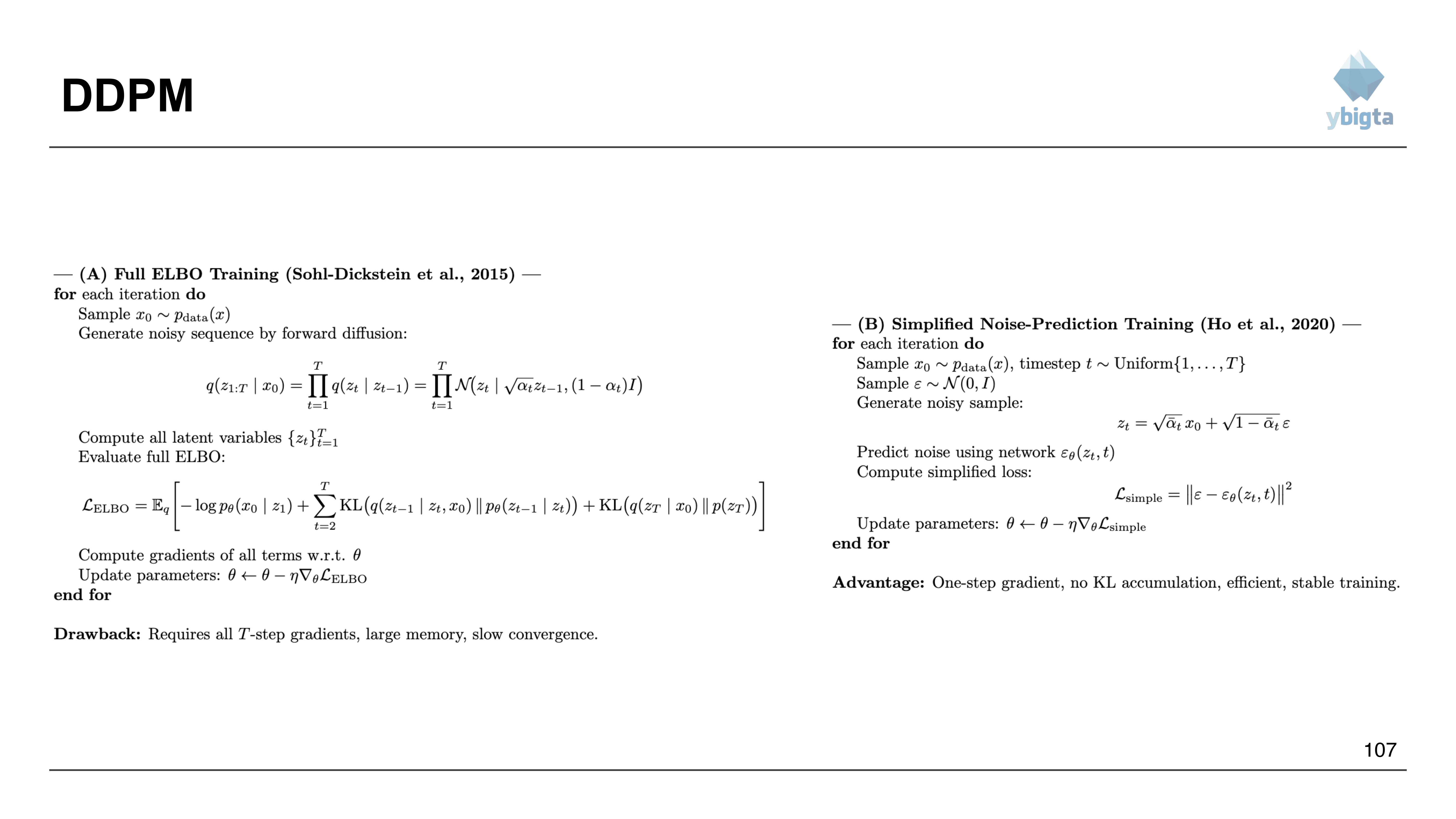
Slide 107: Comparison of Training Methods
- (A) Full ELBO (Sohl-Dickstein): Requires $T$-step gradients, large memory, slow convergence.
- (B) Simplified Noise-Prediction (Ho et al.): One-step gradient (random $t$), no KL accumulation, efficient, stable training.

Slide 108: Conclusion
- Thank You.